Problem Set 4
Please render this file to .html and submit via Brightspace.
Sample mean vs. a reference value
Scenario 1
A marine protected area (MPA) was established five years ago. Previous surveys from nearby fished reefs found a mean fish biomass of 12.2 kg 100m-2.
Researchers survey 15 transects inside the MPA and want to test whether fish biomass is higher than the regional average of fished reefs.
The data are available from the “MPA” sheet in “H2SMS_practicalData.xlsx”. Load and check the data.
tibble [15 × 2] (S3: tbl_df/tbl/data.frame)
 $ transect        : num [1:15] 1 2 3 4 5 6 7 8 9 10 ...
 $ biomass_kg_100m2: num [1:15] 12.8 13.2 12.7 12.6 10.4 ...
Load and check data
summary(MPA_df) transect biomass_kg_100m2
Min. : 1.0 Min. :10.30
1st Qu.: 4.5 1st Qu.:12.14
Median : 8.0 Median :12.79
Mean : 8.0 Mean :12.75
3rd Qu.:11.5 3rd Qu.:13.46
Max. :15.0 Max. :15.02 What is the response variable?
Fish biomass (kg 100m-2)
What is the null hypothesis?
\(\mu_{MPA} \leq 12.2 kg \cdot 100m^{-2}\)
The mean fish biomass within the MPA is less than or equal to the mean fish biomass outside the MPA.
Note that the hypothesis is about the population mean, not the sample mean.
What is the alternative hypothesis?
\(\mu_{MPA} > 12.2 kg \cdot 100m^{-2}\)
The mean fish biomass within the MPA is greater than the mean fish biomass outside the MPA.
Note that the hypothesis is about the population mean, not the sample mean.
Evaluate the null hypothesis using \(\alpha = 0.05\). Perform an appropriate analysis (including assumption checks), and report the relevant results in written text.
Data distribution
pA <- ggplot(MPA_df, aes(biomass_kg_100m2)) +
  geom_histogram(bins=10) +
  geom_rug()
pB <- ggplot(MPA_df, aes(sample=biomass_kg_100m2)) +
  geom_qq() + geom_qq_line() +
  labs(x="Theoretical quantiles",
       y="Observed")
cowplot::plot_grid(pA, pB, nrow=1, align="h", axis="tb")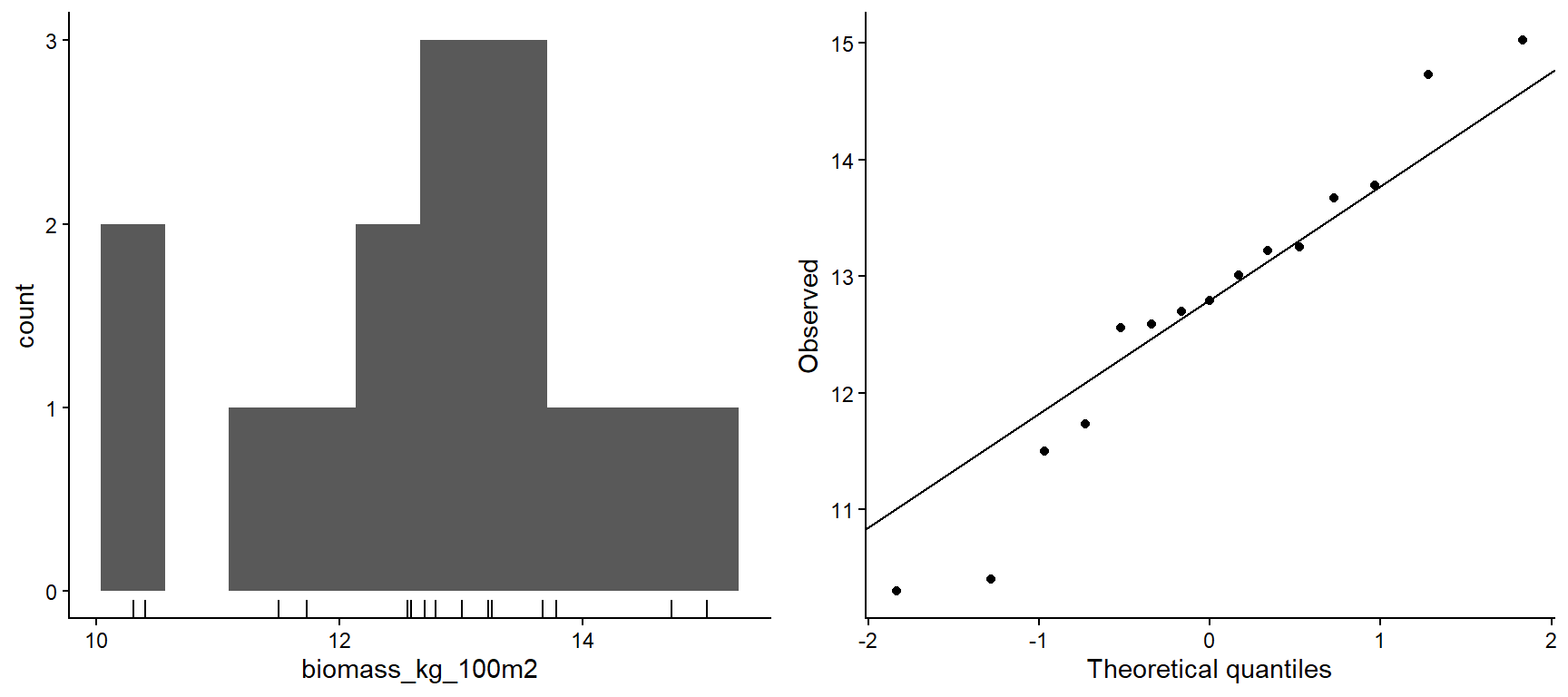
It’s a small sample, but the observations seem approximately normal.
Analysis
t.test(MPA_df$biomass_kg_100m2, mu=12.2, alternative="greater")
    One Sample t-test

data:  MPA_df$biomass_kg_100m2
t = 1.5718, df = 14, p-value = 0.06916
alternative hypothesis: true mean is greater than 12.2
95 percent confidence interval:
 12.13369      Inf
sample estimates:
mean of x
    12.75
In a one-tailed one sample t-test, the mean fish biomass within the MPA (12.8 kg 100m2; 95% confidence limit: 12.1 kg 100m-2) was not significantly greater than the regional mean outside the MPA of 12.2 kg 100m-2 (T14=1.57, p=0.069).
In your own words, explain what the p-value represents.
The p-value gives the probability of these observations if the null hypothesis were true. That is, it is the likelihood of these observed values if the MPA mean were equal to 12.2 kg 100-2.
Scenario 2
In New Zealand, Brewin et al. (2000) studied fecundity and spawning of the sea urchin Evechinus chloroticus, finding a mean annual gamete output of 0.068 g g-1 yr-1 between 1990-1994 at Dieffenbach Point. On my holiday, I decided to repeat that aspect of their experiment (securing all necessary permits and approvals).
The data are in the “UrchinGametes” sheet in “H2SMS_practicalData.xlsx”, already summarised to grams of gamete per grams of urchin per year. Load the data and perform appropriate checks.
Load and check data
tibble [20 × 2] (S3: tbl_df/tbl/data.frame)
 $ urchin_id: num [1:20] 1 2 3 4 5 6 7 8 9 10 ...
 $ output   : num [1:20] 0.0956 0.0476 0.0842 0.0775 0.06 ...
Load and check data
summary(urchin_df) urchin_id output
Min. : 1.00 Min. :0.00359
1st Qu.: 5.75 1st Qu.:0.05743
Median :10.50 Median :0.07049
Mean :10.50 Mean :0.06820
3rd Qu.:15.25 3rd Qu.:0.08477
Max. :20.00 Max. :0.12041 What is the response variable?
Annual gamete output (g gamete per gram of urchin per year)
What is the null hypothesis?
\(\mu_{new} = 0.068 g \cdot g^{-1} \cdot yr^{-1}\)
The mean gamete output of the current population is equal to the historic mean.
Note that the hypothesis is about the population mean, not the sample mean.
What is the alternative hypothesis?
\(\mu_{new} \neq 0.068 g \cdot g^{-1} \cdot yr^{-1}\)
The mean gamete output of the current population is not equal to the historic mean.
Note that the hypothesis is about the population mean, not the sample mean.
Evaluate the null hypothesis using \(\alpha = 0.05\). Perform an appropriate analysis (including assumption checks), and report the relevant results in written text.
Data distribution
pA <- ggplot(urchin_df, aes(output)) +
  geom_histogram(bins=10) +
  geom_rug()
pB <- ggplot(urchin_df, aes(sample=output)) +
  geom_qq() + geom_qq_line() +
  labs(x="Theoretical quantiles",
       y="Observed")
cowplot::plot_grid(pA, pB, nrow=1, align="h", axis="tb")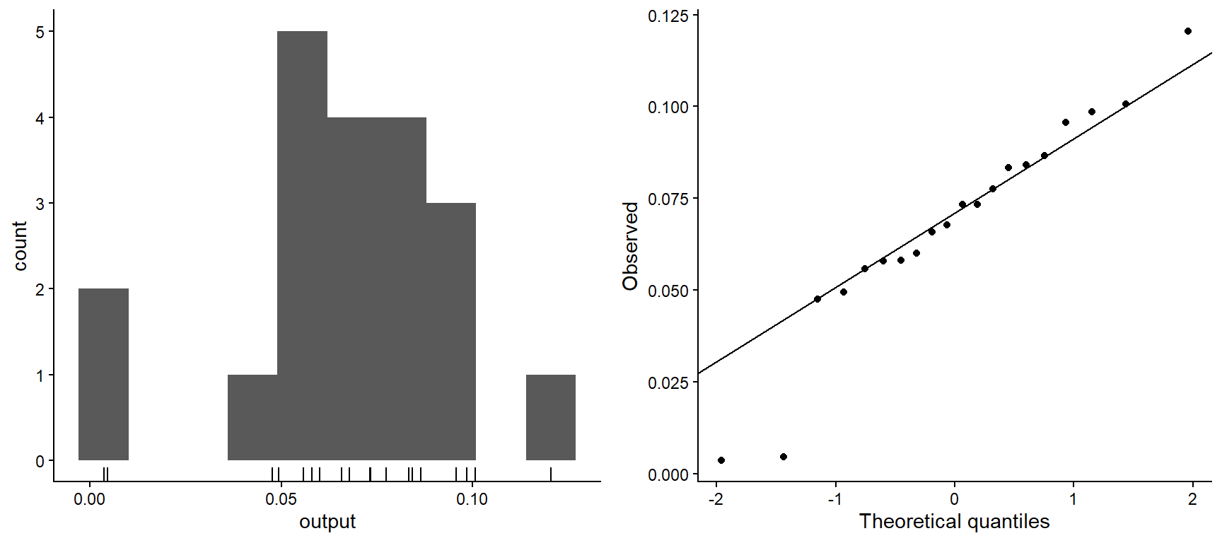
The observations seem approximately normal, given the sample size.
Analysis
t.test(urchin_df$output, mu=0.068)
    One Sample t-test

data:  urchin_df$output
t = 0.030502, df = 19, p-value = 0.976
alternative hypothesis: true mean is not equal to 0.068
95 percent confidence interval:
 0.05467906 0.08171494
sample estimates:
mean of x
 0.068197
In a two-tailed one sample t-test, the mean gamete output (0.0682 g g-1 yr-1; 95% CI: 0.0547-0.0817 g g-1 yr-1) was not significantly different than the historic average of 0.068 g g-1 yr-1 (T19=0.03, p=0.976).
In your own words, interpret your results with regard to the null hypothesis and the p-value.
The observed gamete output was entirely plausible under the null hypothesis that the population mean was the same as in 1990-1994.
Confidence Intervals
The sheet “Plastics” in “H2SMS_practicalData.xlsx” contains observations of the number of plastic pellets per kilogram. Load the data.
Load and check data
tibble [100,000 × 2] (S3: tbl_df/tbl/data.frame)
 $ id     : num [1:100000] 1 2 3 4 5 6 7 8 9 10 ...
 $ pellets: num [1:100000] 431 673 548 560 429 498 406 591 438 406 ...
Load and check data
summary(plastic_df) id pellets
Min. : 1 Min. : 66.0
1st Qu.: 25001 1st Qu.:432.0
Median : 50001 Median :500.0
Mean : 50001 Mean :499.7
3rd Qu.: 75000 3rd Qu.:567.0
Max. :100000 Max. :924.0 Consider this the entire population of interest.
Write code to take a sample of 25 observations from this population and store it in a vector called obs.
View code
obs <- sample(plastic_df$pellets, size=25)How different is your sample mean from the true population mean?
What is the term that describes this difference?
Sampling error: The difference between a sample statistic and the population parameter.
Calculate 95% confidence intervals for your sample mean using only your sample. Do they include the true value?
The easy way
t.test(obs)
    One Sample t-test

data:  obs
t = 20.866, df = 24, p-value < 2.2e-16
alternative hypothesis: true mean is not equal to 0
95 percent confidence interval:
 446.3995 544.4005
sample estimates:
mean of x
    495.4
The hard way
[1] 446.3995 544.4005In this case, yes.
Assuming each student starts with a different set.seed, what proportion of students would answer ‘yes’ to the previous question?
0.95 = 95%
If you instead calculated 80% CIs, a) would you be more likely to capture the true mean or less? And, b) would the width of your confidence interval be larger or smaller?
- Less likely and b) smaller. An 80% CI will only include the true value in 80% of samples (under ideal conditions!), while a 95% CI will include the true value in 95% of samples.
Calculate the 80% CI for your sample and compare.
[1] 446.3995 544.4005
attr(,"conf.level")
[1] 0.95
View code
ci_80[1] 464.1123 526.6877
attr(,"conf.level")
[1] 0.8View code
expand_grid(confidence=c(0.8, 0.95),
            limit=c("lo", "high")) |>
  mutate(limit=c(ci_80, ci_95)) |>
  ggplot(aes(limit, confidence, group=confidence)) +
  geom_line() +
  geom_point(shape="|") +
  geom_vline(xintercept=mean(plastic_df$pellets), linetype=3) +
  labs(x="Value", y="Confidence level")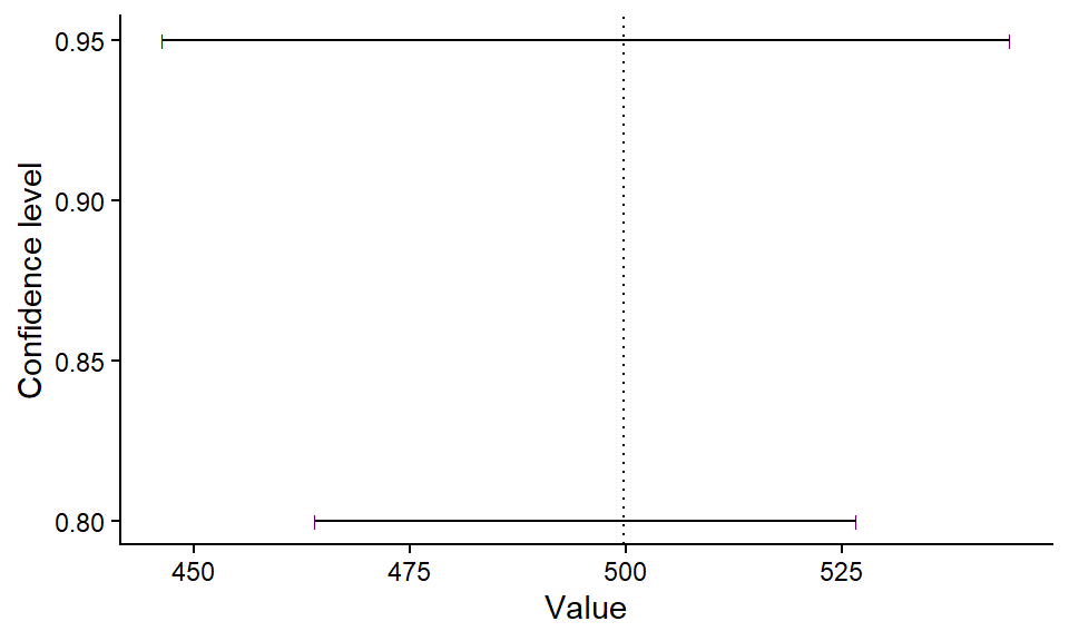
If you were to run your code again (without resetting set.seed), what is the probability that you would collect a sample with a 90% CI that includes the true value?
90% - each (future) sample will have a 90% chance of having 90% CIs that include the true value.