Problem Set 3

Please render this file to .html and submit via Brightspace.

library(tidyverse); theme_set(theme_classic())
library(readxl)
set.seed(2026)

Normal distribution

Scenario 1: Using `*norm()`

For a particular population of brown seaweed, the winter carbon:nitrogen ratio is distributed approximately normally among individuals as \(y \sim Norm(\mu=27.6, \sigma=2.5)\).

What proportion of the population would you expect to have a C:N ratio greater than 30?

Proportion > 30

mu <- 27.6
sigma <- 2.5

1 - pnorm(30, mu, sigma)

[1] 0.1685276

What is the probability of sampling an individual with a ratio between 23 and 24?

Pr(23 < y < 24)

pnorm(24, mu, sigma) - pnorm(23, mu, sigma)

[1] 0.04204958

What ratio would delineate the lowest 30% of the population?

Lowest 30%

qnorm(0.3, mu, sigma)

[1] 26.289

Generate a random sample of 12 individuals from this population. Calculate the sample mean and sample standard deviation.

Collect a random sample

obs <- rnorm(12, mu, sigma)

Sample mean and sd

# Mean:
mean(obs)

# sd:
sd(obs)

[1] 26.15386
[1] 1.957169

What is the difference between your sample mean and the true population mean called? Why does it occur and what are two aspects of your sampling design that affect it?

Definition

# This is sampling error: the difference between the true population parameter
# and the statistic calculated from a sample. It is inevitable that a statistic
# from a sample (e.g., a sample mean) will be different from the parameter for
# the entire population (e.g., the population mean) because a sample is only
# a subset of the whole population.

Sampling impact 1

# Sampling error is strongly affected by:
# 1) Sample size: A larger sample will, on average, have smaller sampling error
#     since differences among individuals 'average out'

Sampling impact 2

# Sampling error is strongly affected by:
# 2) Randomization: A non-random sample introduces bias, making some individuals
#     more likely to be included. This bias will tend to make sampling error 
#     biased as well.

Sampling impact 3

# Sampling error is strongly affected by:
# 3) Population variability: A more variable population (larger sigma) means the
#     observations in a sample are more variable, and so sampling error will
#     tend to be larger. Standardizing conditions as much as possible can reduce
#     this source of noise.

Repeat your random sampling 1000 times, calculate a sample mean for each of the 1000 samples, and make a histogram of them. Calculate the mean of these sample means.

Hint

# y_bar <- rep(0, 1000)
# for(i in 1:1000) {
#   y_bar[i] <- ...
# }

Repeated sampling

y_bar <- rep(0, 1000)
for(i in 1:1000) {
  y_bar[i] <- mean(rnorm(12, mu, sigma))
}

Histogram (ggplot)

tibble(y_bar=y_bar) |>
  ggplot(aes(y_bar)) +
  geom_histogram(bins=15, colour="black", fill="grey") +
  geom_vline(xintercept=mu, colour="blue")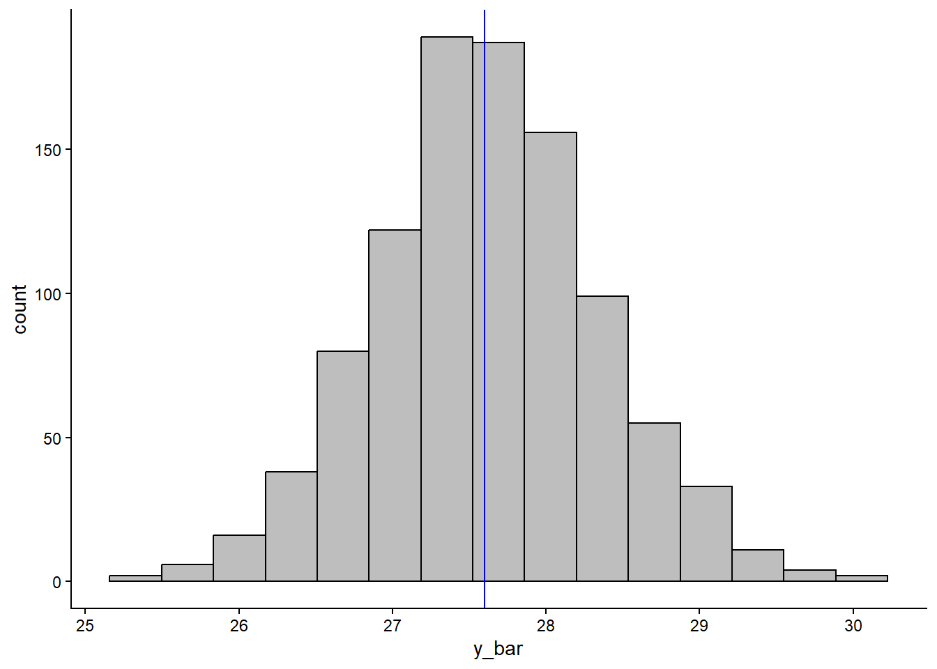

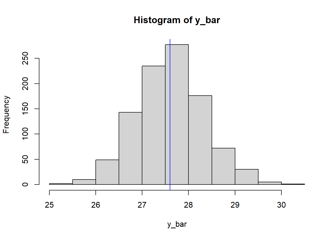
Histogram (base R)

hist(y_bar, breaks=15); abline(v=mu, col="blue")

Mean of sample means

signif(mean(y_bar), 3)

[1] 27.6

How does this mean (and the histogram) compare to the population mean?

Comparison sample means vs. mu

# The mean of sample means is very close to mu, and the histogram of sample means
# is centred on mu. 
#
# Note also that the distribution is approximately normal, illustrating the 
# Central Limit Theorem (since the population is ~Norm).
# 
# This relies on a *random* sample. If the sampling is biased (non-random), this
# pattern can not be relied upon!

Scenario 2: Transformations

The swiss dataset in R gives standardised fertility and socioeconomic indicators for each of the 47 French-speaking provinces of Switzerland in ca. 1888:

str(swiss)

'data.frame':   47 obs. of  6 variables:
 $ Fertility       : num  80.2 83.1 92.5 85.8 76.9 76.1 83.8 92.4 82.4 82.9 ...
 $ Agriculture     : num  17 45.1 39.7 36.5 43.5 35.3 70.2 67.8 53.3 45.2 ...
 $ Examination     : int  15 6 5 12 17 9 16 14 12 16 ...
 $ Education       : int  12 9 5 7 15 7 7 8 7 13 ...
 $ Catholic        : num  9.96 84.84 93.4 33.77 5.16 ...
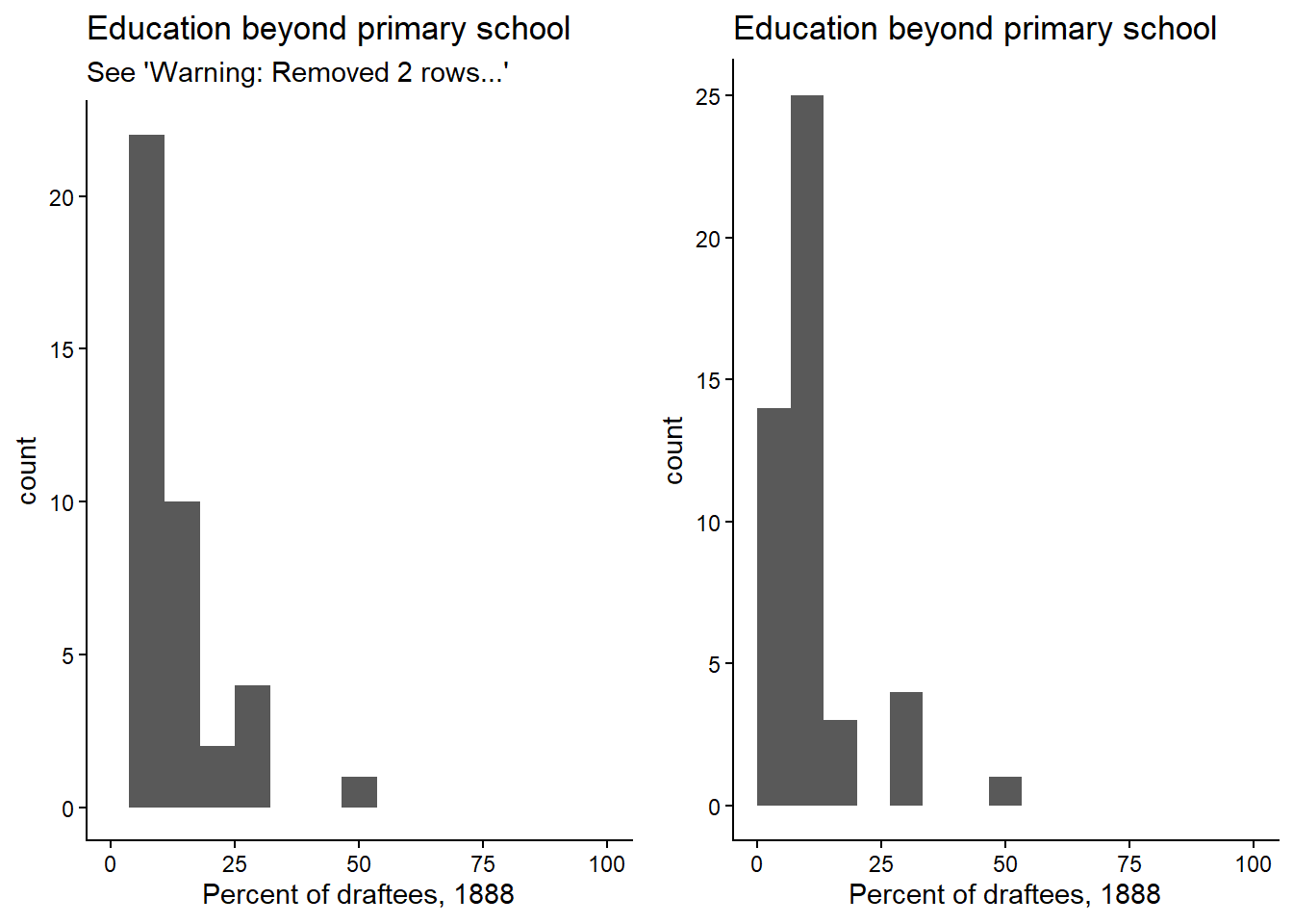
 $ Infant.Mortality: num  22.2 22.2 20.2 20.3 20.6 26.6 23.6 24.9 21 24.4 ...

The values are given as percentages ranging from 0-100. Make a histogram for the Education column, setting the x-axis limits to the theoretical range of the variable.

Histogram (ggplot)

cowplot::plot_grid(
  # default geom_histogram() settings: Notice that the 0's get dropped when 
  # setting xlim(0, 100)! This is because by default the bars were centred
  # on 0, and so setting xlim(0,...) means it can't draw the left half of the
  # bar, so it drops it. At least there is a warning...
  ggplot(swiss, aes(Education)) +
    geom_histogram(bins=15) +
    xlim(0, 100) +
    labs(title="Education beyond primary school",
         subtitle="See 'Warning: Removed 2 rows...'",
         x="Percent of draftees, 1888"),
  # to avoid this, we can set 'boundary=0' to make 0 the boundary for the bar
  # rather than the centre. In this case, 0 is a theoretical limit, but ggplot
  # doesn't know that.
  ggplot(swiss, aes(Education)) +
    xlim(0, 100) +
    geom_histogram(bins=15, boundary=0) +
    labs(title="Education beyond primary school",
         x="Percent of draftees, 1888")
)

Histogram (base R)

hist(swiss$Education, 
     xlim=c(0, 100),
     breaks=14,
     main="Education beyond primary school",
     xlab="Percent of draftees, 1888")

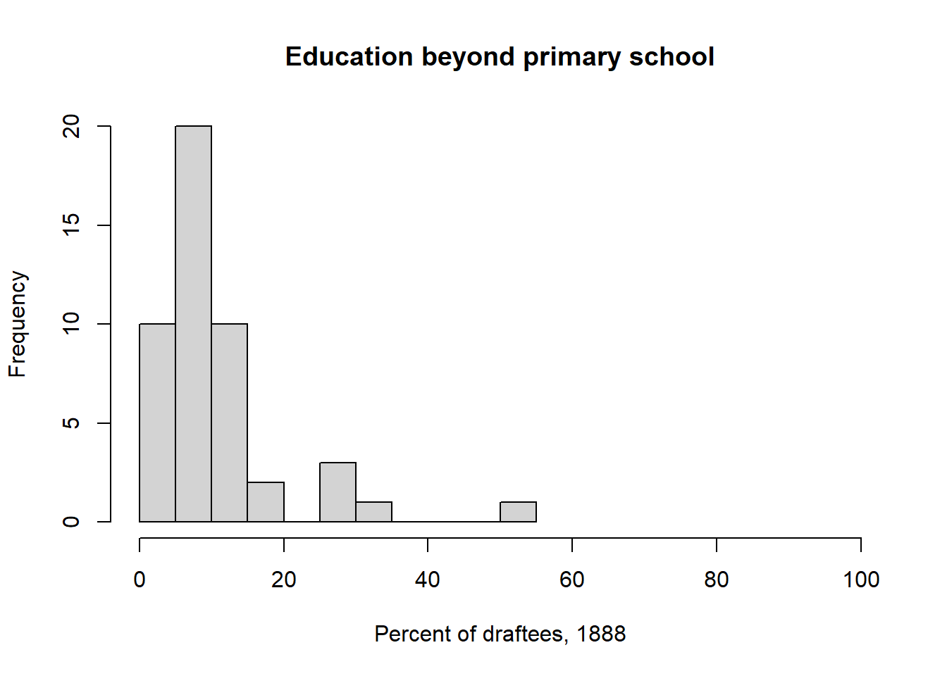
What transformation would be most appropriate for these kinds of data?

Solution

# Logistic: Data are percentages (convert to proportions by dividing by 100) 
# and tend to be smaller values near the lower boundary (0%) with a long tail 
# of larger values (right skew).

# A log transformation may also be suitable.

Apply this transformation and make a histogram of the transformed values.

Transformation and histogram (ggplot)

ggplot(swiss, aes(boot::logit(Education/100))) +
  geom_histogram(bins=8) + 
  labs(title="Education beyond primary school",
       x="logit(Proportion of draftees), 1888")

Transformation and histogram (base R)

hist(boot::logit(swiss$Education/100), 
     breaks=8,
     main="Education beyond primary school",
     xlab="logit(Proportion of draftees), 1888")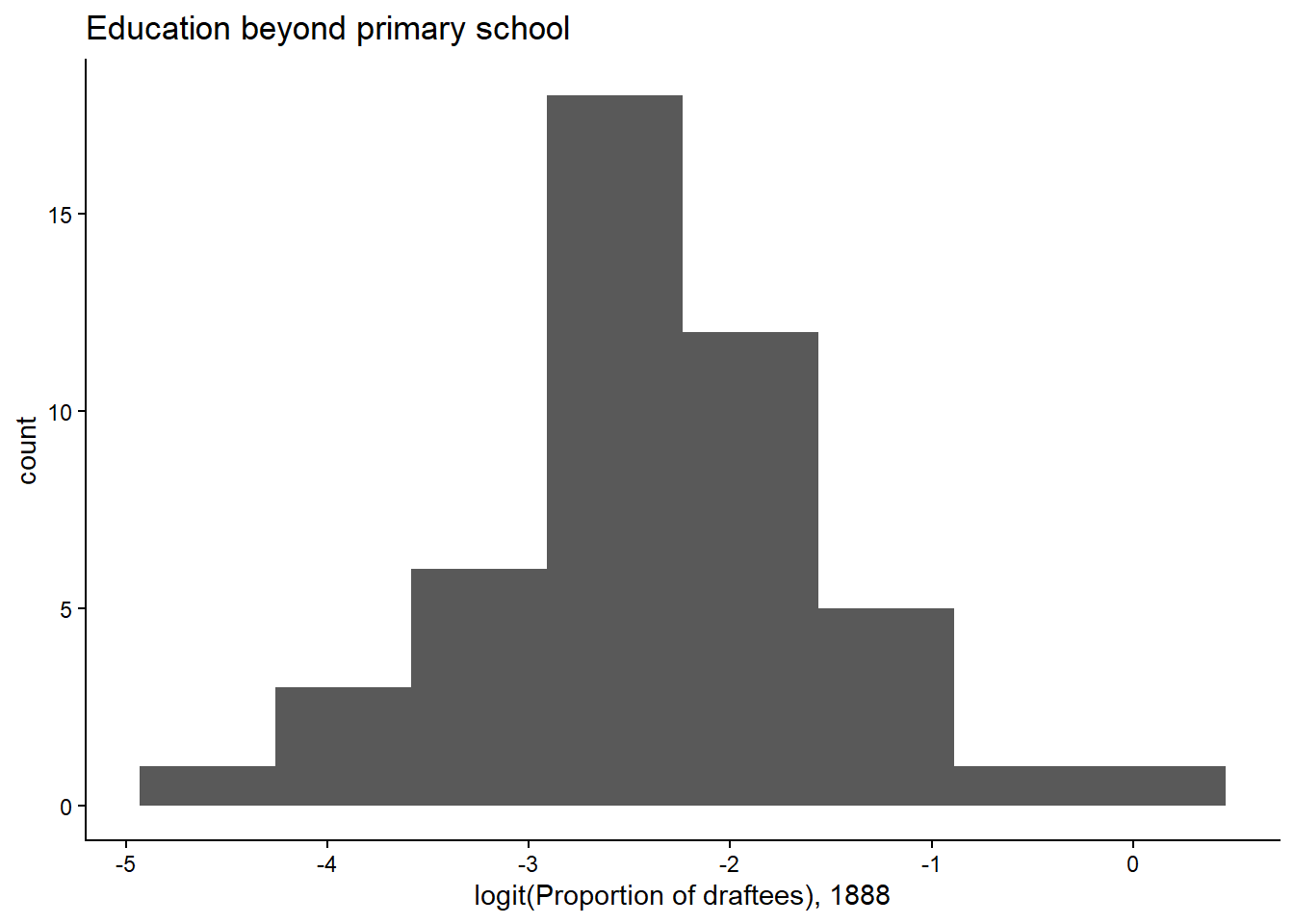

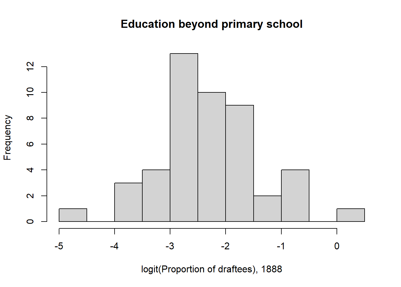
What do you notice about the shape of the original and transformed distributions?

Solution

# The transformed distribution looks much more like a normal distribution.

Standard error of the mean

For the seaweed population in Scenario 1, we simulated a sample of 12 individuals from the population. In my particular sample, I found a sample mean of 26.154. Recall that the true population was distributed as \(y \sim Norm(\mu=27.6, \sigma=2.5)\).

Using the true population standard deviation \(\sigma=2.5\), calculate the standard error of the mean.

Solution

sigma <- 2.5
n <- 12

sigma / sqrt(n)

[1] 0.7216878

In your own words, describe what the standard error of the mean is.

Solution (my words)

# The standard error of the mean is the standard deviation of the distribution 
# of possible sample means from a given population. It describes the breadth 
# of the distribution of sample means we would expect if we were to collect 
# many, many different samples, each with size n, and calculate a mean from 
# each sample.

The distribution of sample means can be simulated in R. Write code to 1) simulate 100 different samples from the seaweed population with \(n=12\), and 2) calculate a sample mean from each of these 100 samples.

Solution

n_samples <- 100
n <- 12
sample_means <- rep(0, n_samples)
for(i in 1:n_samples) {
  sample_means[i] <- rnorm(n, mu, sigma) |> mean()
}

Make a plot to show the distribution of these sample means, and indicate the true population mean \(\mu\).

Solution (ggplot)

tibble(sample_means=sample_means) |>
  ggplot(aes(sample_means)) + 
  geom_histogram(bins=10) + 
  geom_vline(xintercept=mu, colour="red", linewidth=2)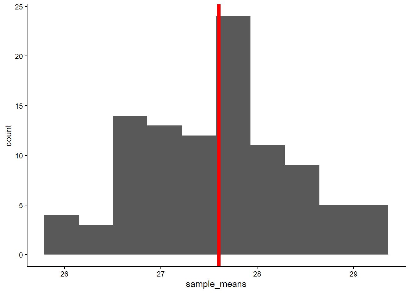

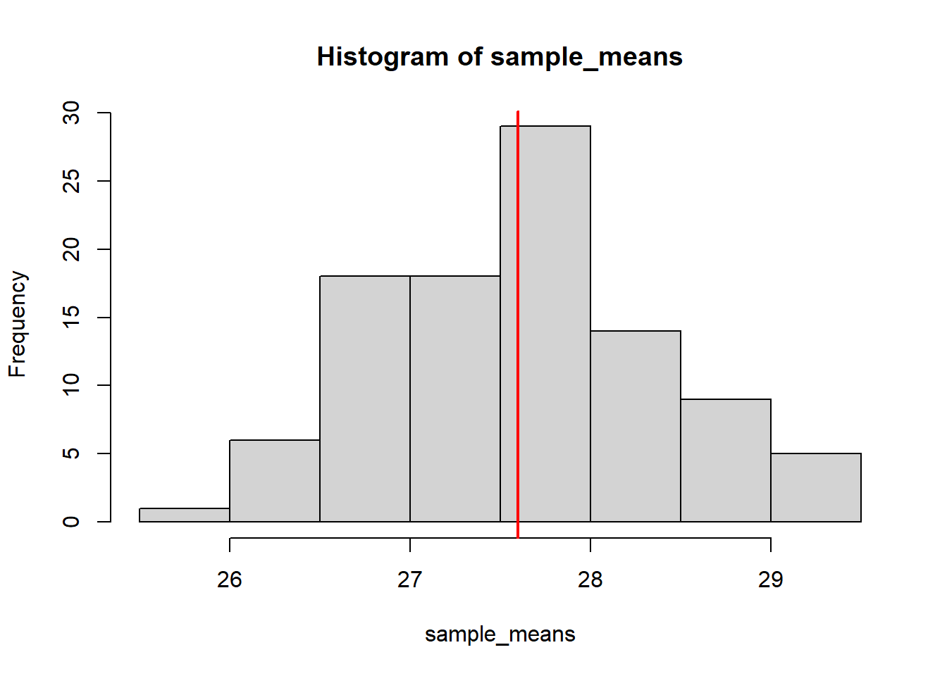
Solution (base R)

hist(sample_means, breaks=10)
abline(v=mu, col="red", lwd=2)

Calculate the standard deviation of the 100 sample means.

Solution

sd(sample_means)

[1] 0.7922183

How does it compare to the standard error of the mean you calculated above? Try increasing the number of samples to 3,000 and recalculate.

Solution

# The standard deviation of the sample means should be close. Increasing the 
# number of samples should bring this value even closer to the standard error 
# of the mean calculated analytically. Note that this is because we are 
# averaging over sampling error!

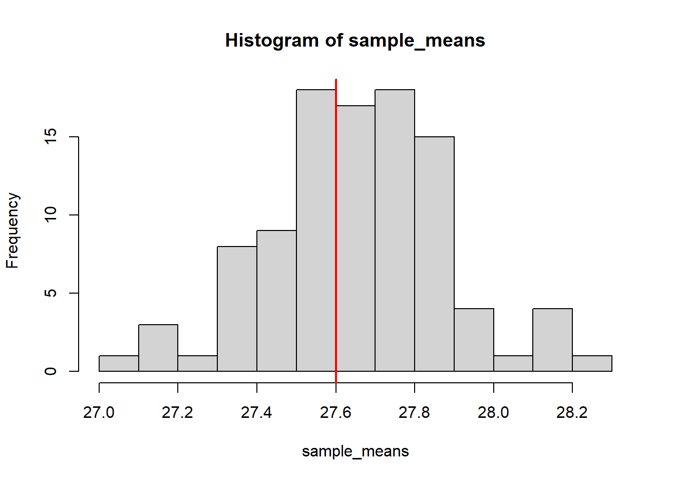
Lastly, repeat the process, this time with \(n=120\) for each sample. Calculate the standard error of the mean, simulate 100 sample means, and compare the standard deviation of these with the calculated standard error.

Solution

n <- 120

sigma / sqrt(n)

[1] 0.2282177

Solution

n_samples <- 100
sample_means <- rep(0, n_samples)
for(i in 1:n_samples) {
  sample_means[i] <- rnorm(n, mu, sigma) |> mean()
}
sd(sample_means)

[1] 0.2279312

Histogram (ggplot)

tibble(sample_means=sample_means) |>
  ggplot(aes(sample_means)) + 
  geom_histogram(bins=10) + 
  geom_vline(xintercept=mu, colour="red", linewidth=2)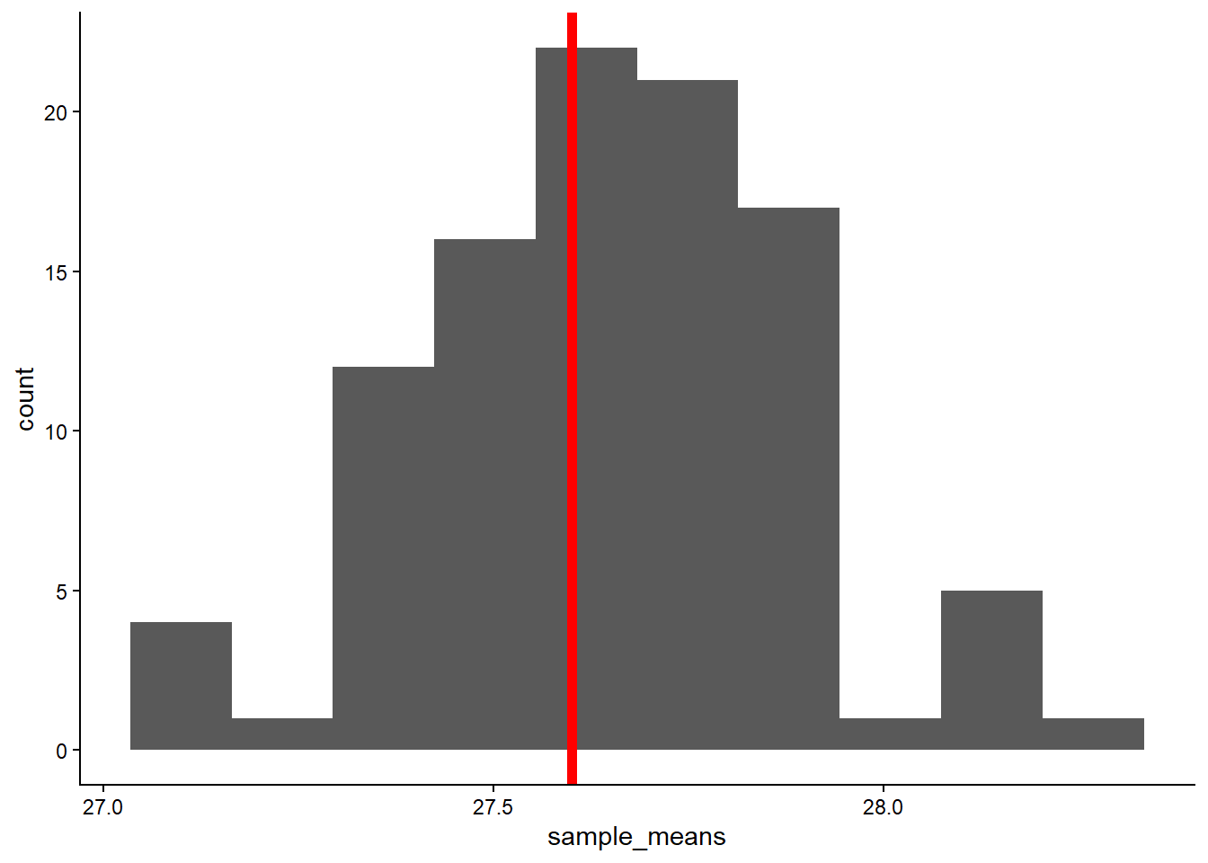

Histogram (base R)

hist(sample_means, breaks=10)
abline(v=mu, col="red", lwd=2)

Why does the standard error decrease? What does this tell us about our level of confidence in the sample statistics we calculate (\(\bar{y}\), \(s\)) and our inferences about the population parameters we are interested in (\(\mu\), \(\sigma\))?

Solution

# Sample means will vary less (among samples) as the size of each sample 
# increases. The variability among individuals averages out, and our samples 
# become more representative of the population. According to the equation, the 
# standard error decreases with the square root of the sample size. 

# So, with a larger sample size, we can be more confident that our sample mean 
# is near to the population mean. 

# Note that this assumes proper sampling methodology! 
# (See Experimental Design lectures)

Normal distribution

Scenario 1: Using *norm()

Scenario 2: Transformations

Standard error of the mean

Scenario 1: Using `*norm()`