Extra: CA1

View original

Download file

Overview

Coverage: L01-L09, P1-P3

This is a document to give you additional practice working in R. It will include working with data (manipulating, summarising, plotting) and analyzing the distributions we’ve covered.

Please do not treat this as a comprehensive study guide for CA1!

Note that there are often many possible paths to the correct solution.

library(tidyverse); theme_set(theme_classic())
library(readxl)
set.seed(2026)

Iris

The iris dataset is available in R upon start-up.

What are the dimensions of the object (rows, columns) and what data type is it?

str(iris)

'data.frame':   150 obs. of  5 variables:
 $ Sepal.Length: num  5.1 4.9 4.7 4.6 5 5.4 4.6 5 4.4 4.9 ...
 $ Sepal.Width : num  3.5 3 3.2 3.1 3.6 3.9 3.4 3.4 2.9 3.1 ...
 $ Petal.Length: num  1.4 1.4 1.3 1.5 1.4 1.7 1.4 1.5 1.4 1.5 ...
 $ Petal.Width : num  0.2 0.2 0.2 0.2 0.2 0.4 0.3 0.2 0.2 0.1 ...
 $ Species     : Factor w/ 3 levels "setosa","versicolor",..: 1 1 1 1 1 1 1 1 1 1 ...

Create a scatter plot of sepal area on the x-axis and petal area on the y-axis.

First create new columns Sepal.Area and Petal.Area.

# method 1
iris_df <- iris |>
  mutate(Sepal.Area=Sepal.Length*Sepal.Width,
         Petal.Area=Petal.Length*Petal.Width)

# method 2
iris_df <- iris
iris$Sepal.Area <- iris$Sepal.Length * iris$Sepal.Width
iris$Petal.Area <- iris$Petal.Length * iris$Petal.Width

Then make the scatter plot:

plot(Petal.Area ~ Sepal.Area, data=iris)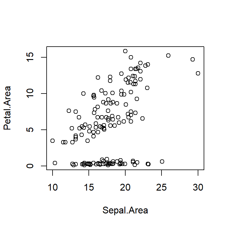

For each species, what is the mean and standard deviation of sepal area?

# method 1
iris |>
  group_by(Species) |>
  summarise(mean_SepalArea=mean(Sepal.Area),
            sd_SepalArea=sd(Sepal.Area))

# A tibble: 3 × 3
  Species    mean_SepalArea sd_SepalArea
  <fct>               <dbl>        <dbl>
1 setosa               17.3         2.93
2 versicolor           16.5         2.87
3 virginica            19.7         3.46

# method2
summary(iris$Species) # unique values of Species
mean(iris$Sepal.Area[iris$Species=="setosa"])
mean(iris$Sepal.Area[iris$Species=="versicolor"])
mean(iris$Sepal.Area[iris$Species=="virginica"])
sd(iris$Sepal.Area[iris$Species=="setosa"])
sd(iris$Sepal.Area[iris$Species=="versicolor"])
sd(iris$Sepal.Area[iris$Species=="virginica"])

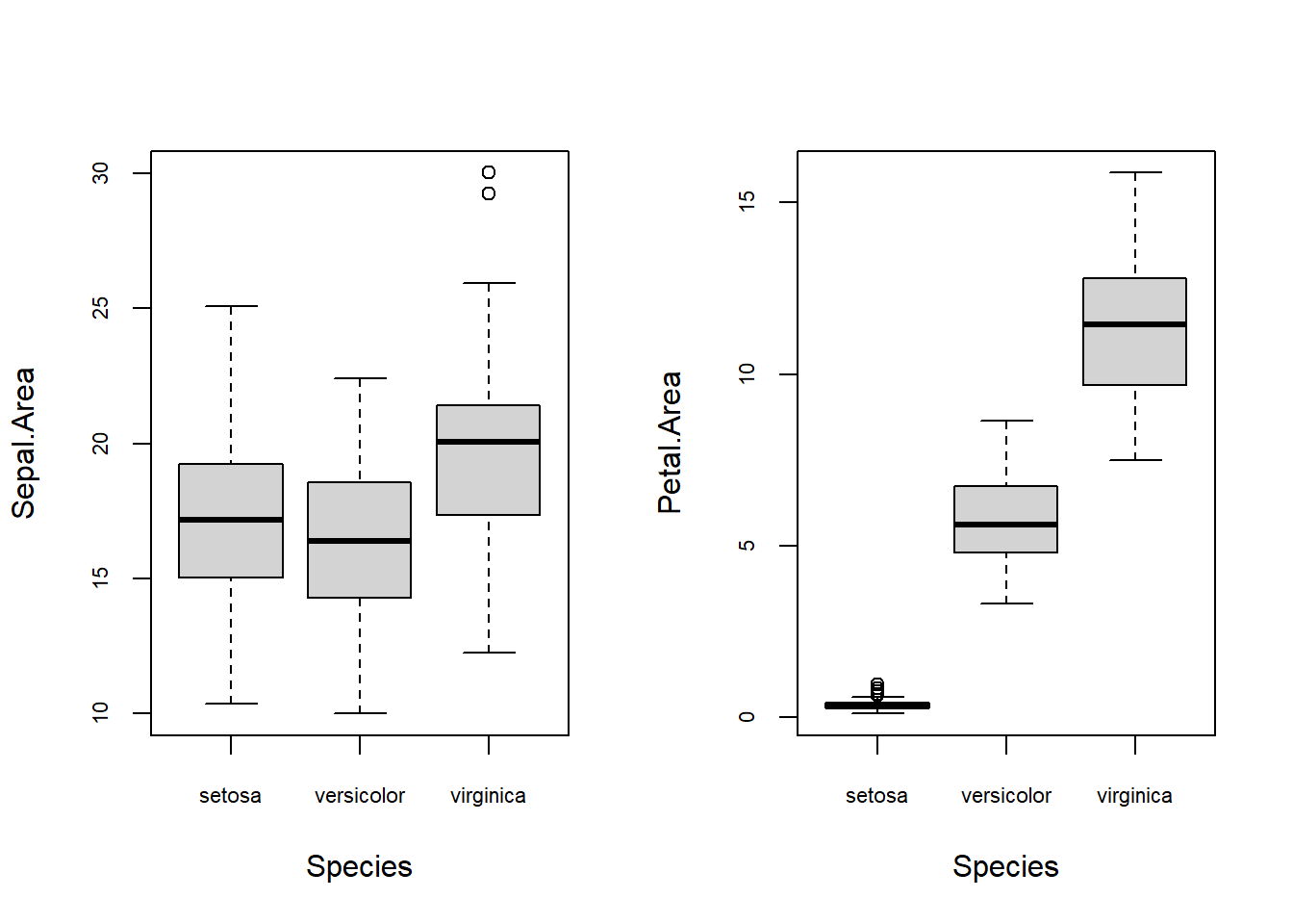
Create a plot with two panels, each with a boxplot with species on the x-axis. In the first panel, plot sepal area on the y-axis. In the second panel, plot petal area on the y-axis.

par(mfrow=c(1,2))
boxplot(Sepal.Area ~ Species, data=iris, cex.axis=0.7)
boxplot(Petal.Area ~ Species, data=iris, cex.axis=0.7)

Extract the even numbered rows from iris, and the columns Species, Sepal.Area, and Petal.Area in that order.

iris[seq(2, nrow(iris), by=2), c("Species", "Sepal.Area", "Petal.Area")]

       Species Sepal.Area Petal.Area
2       setosa      14.70       0.28
4       setosa      14.26       0.30
6       setosa      21.06       0.68
8       setosa      17.00       0.30
10      setosa      15.19       0.15
12      setosa      16.32       0.32
14      setosa      12.90       0.11
16      setosa      25.08       0.60
18      setosa      17.85       0.42
20      setosa      19.38       0.45
22      setosa      18.87       0.60
24      setosa      16.83       0.85
26      setosa      15.00       0.32
28      setosa      18.20       0.30
30      setosa      15.04       0.32
32      setosa      18.36       0.60
34      setosa      23.10       0.28
36      setosa      16.00       0.24
38      setosa      17.64       0.14
40      setosa      17.34       0.30
42      setosa      10.35       0.39
44      setosa      17.50       0.96
46      setosa      14.40       0.42
48      setosa      14.72       0.28
50      setosa      16.50       0.28
52  versicolor      20.48       6.75
54  versicolor      12.65       5.20
56  versicolor      15.96       5.85
58  versicolor      11.76       3.30
60  versicolor      14.04       5.46
62  versicolor      17.70       6.30
64  versicolor      17.69       6.58
66  versicolor      20.77       6.16
68  versicolor      15.66       4.10
70  versicolor      14.00       4.29
72  versicolor      17.08       5.20
74  versicolor      17.08       5.64
76  versicolor      19.80       6.16
78  versicolor      20.10       8.50
80  versicolor      14.82       3.50
82  versicolor      13.20       3.70
84  versicolor      16.20       8.16
86  versicolor      20.40       7.20
88  versicolor      14.49       5.72
90  versicolor      13.75       5.20
92  versicolor      18.30       6.44
94  versicolor      11.50       3.30
96  versicolor      17.10       5.04
98  versicolor      17.98       5.59
100 versicolor      15.96       5.33
102  virginica      15.66       9.69
104  virginica      18.27      10.08
106  virginica      22.80      13.86
108  virginica      21.17      11.34
110  virginica      25.92      15.25
112  virginica      17.28      10.07
114  virginica      14.25      10.00
116  virginica      20.48      12.19
118  virginica      29.26      14.74
120  virginica      13.20       7.50
122  virginica      15.68       9.80
124  virginica      17.01       8.82
126  virginica      23.04      10.80
128  virginica      18.30       8.82
130  virginica      21.60       9.28
132  virginica      30.02      12.80
134  virginica      17.64       7.65
136  virginica      23.10      14.03
138  virginica      19.84       9.90
140  virginica      21.39      11.34
142  virginica      21.39      11.73
144  virginica      21.76      13.57
146  virginica      20.10      11.96
148  virginica      19.50      10.40
150  virginica      17.70       9.18

Air quality

The airquality dataset is available in R upon start-up, and gives daily values of mean ozone, solar radiation, mean wind speed, and max temperature at LaGuardia Airport in New York City (?airquality).

Make a histogram of wind speed.

hist(airquality$Wind)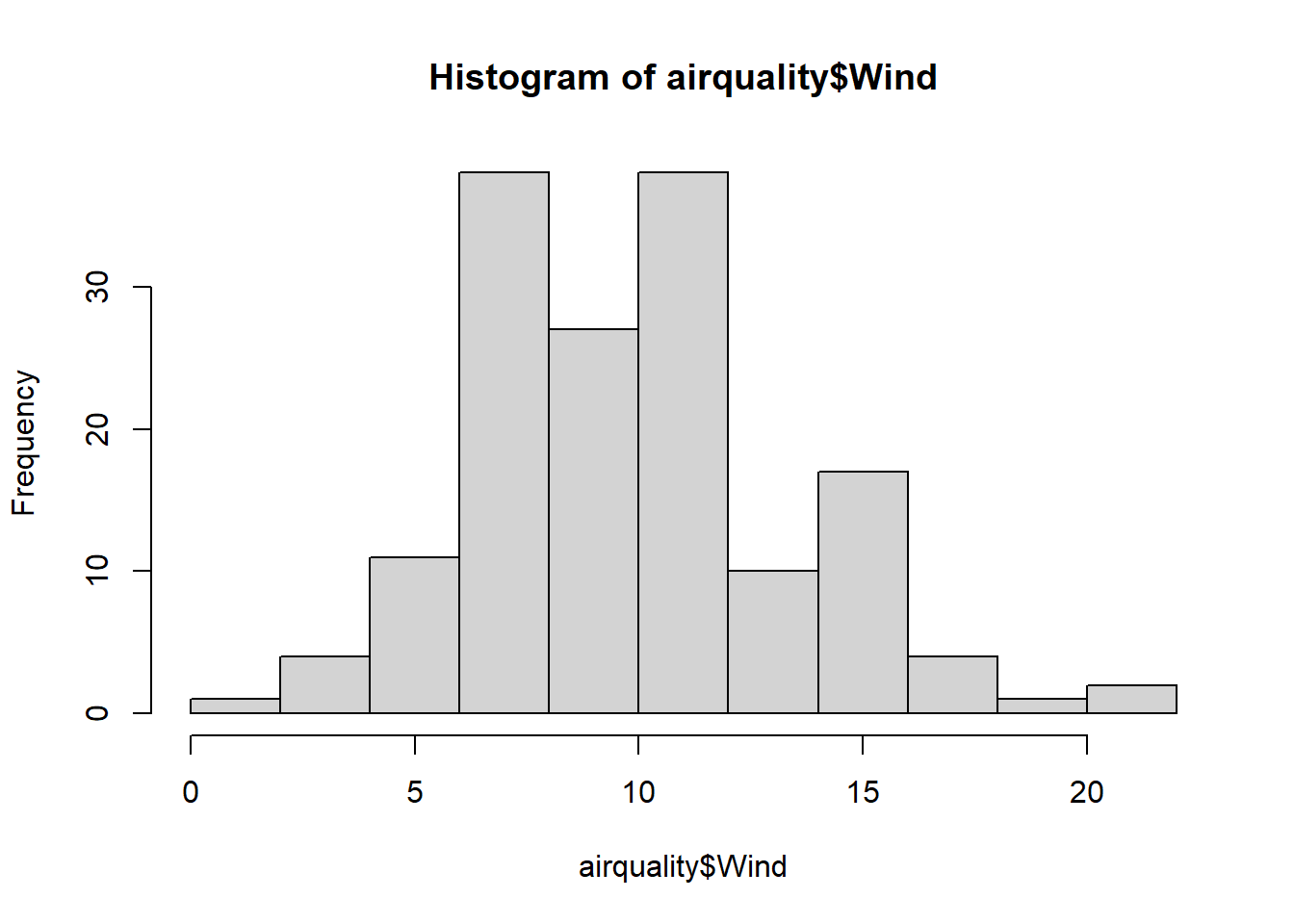

Assume wind speed is normally distributed in this dataset with \(\mu=9.99 mph\) and \(\sigma = 3.51 mph\).

What proportion of days would you expect to have a wind speed less than 5 mph?

pnorm(5, 9.99, 3.51)

[1] 0.07756359

You have a kite that can only be flown safely in winds between 14 mph and 20 mph. What proportion of days would be suitable?

pnorm(20, 9.99, 3.51) - pnorm(14, 9.99, 3.51)

[1] 0.1244602

How many days would be suitable in a 31-day month?

31 * (pnorm(20, 9.99, 3.51) - pnorm(14, 9.99, 3.51))

[1] 3.858267

What proportion of days in the dataset were actually suitable?

mean(airquality$Wind >= 14 & airquality$Wind <= 20)

[1] 0.1437908

What are the z-scores for 14 and 20 mph?

(14 - 9.99)/3.51

[1] 1.14245

(20 - 9.99)/3.51

[1] 2.851852

What are the quantiles for the middle 95%?

qnorm(c(0.025, 0.975), 9.99, 3.51)

[1]  3.110526 16.869474

What is the quantile for the largest 5%?

qnorm(0.95, 9.99, 3.51)

[1] 15.76344

Given the population parameters above, what is the z score of the sample mean in the dataset?

(mean(airquality$Wind) - 9.99)/(3.51/sqrt(nrow(airquality)))

[1] -0.1144731

Given the population parameters above, what is the probability of observing a sample mean smaller than the one in this dataset?

pnorm(mean(airquality$Wind), 9.99, 3.51/sqrt(nrow(airquality)))

[1] 0.4544314

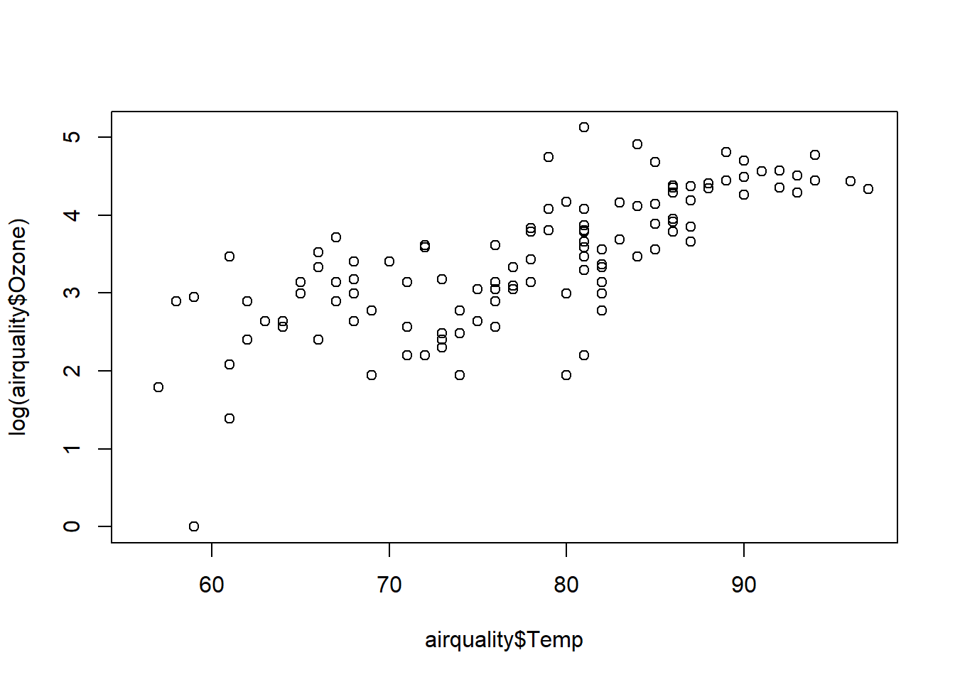
Create a scatter plot with temperature on the x-axis and log-transformed ozone on the y-axis.

plot(airquality$Temp, log(airquality$Ozone))

Create a boxplot with the solar radiation on the y-axis and the month on the x-axis.

boxplot(Solar.R ~ Month, data=airquality)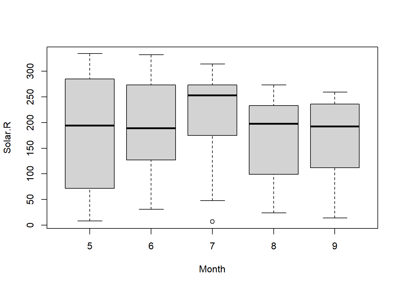

Coral predation

You are studying predation of the Flamingo Tongue Snail on soft corals on South Water Caye in Belize. In a distinct patch of reef, you randomly select a sample of 14 corals and identify that 9 of these have feeding scars.

What distribution would you expect this variable (i.e., the number of corals with feeding scars of those sampled) to follow?

Binomial

What is your sample proportion and its standard error?

p_hat <- 9/14
p_hat

[1] 0.6428571

sqrt((p_hat)*(1-p_hat)/(14-1))

[1] 0.1328944

Create a bar graph of the binomial distribution corresponding to these parameters, with the x-axis spanning the full range of possible outcomes.

barplot(dbinom(0:14, 14, prob=9/14), names.arg=0:14)

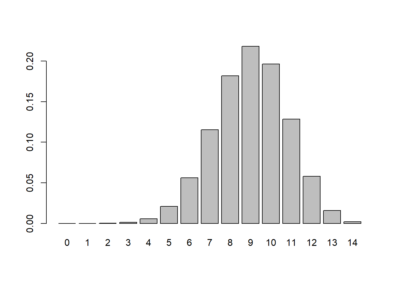
Based on this distribution, if you were to collect another random sample of the same size, what is the probability that all 14 would have feeding scars?

dbinom(14, 14, 9/14)

[1] 0.002058745

What is the probability you would find fewer with feeding scars than in the first sample?

pbinom(8, 14, 9/14)

[1] 0.3811746

What is the probability of finding more with feeding scars than in the first sample?

1-pbinom(9, 14, 9/14)

[1] 0.400701

What is the probability of a sample with 4, 5, or 6 corals with feeding scars?

sum(dbinom(4:6, 14, 9/14))

[1] 0.08265225

Earthquakes

The dataset quakes is available in R upon start-up, and gives magnitudes and locations for 1000 seismic events near Fiji since 1964.

Plot the locations of the earthquakes (x-axis: longitude, y-axis: latitude).

plot(lat ~ long, data=quakes)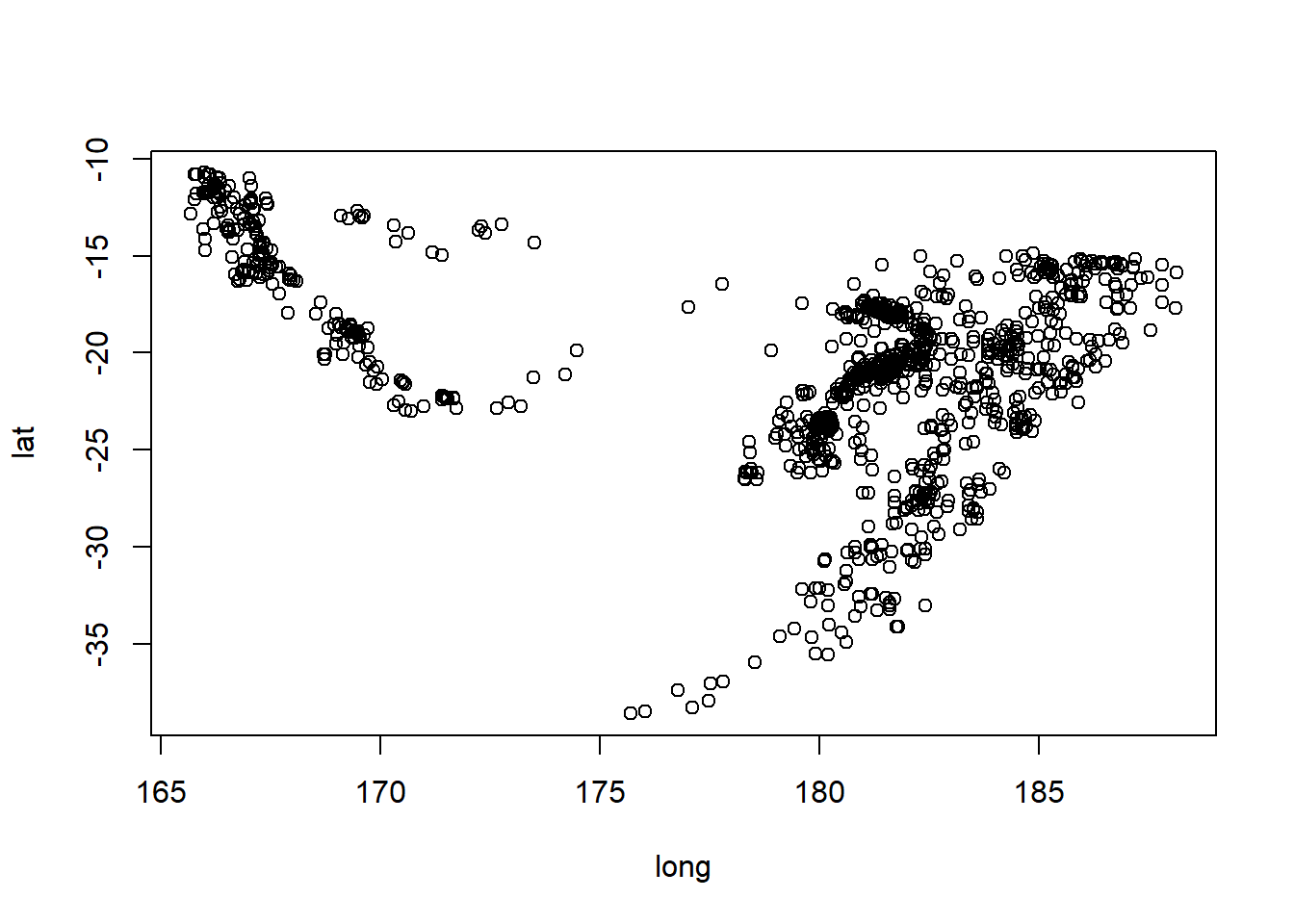

Create a column called mag_cat with the magnitude truncated to integer (i.e., 4.0-4.99 become 4). Hint: ?trunc

quakes$mag_cat <- trunc(quakes$mag)

For each magnitude category (mag_cat), count the number of occurrences in the dataset.

summary(quakes) # ranges 3-6

      lat              long           depth            mag      
 Min.   :-38.59   Min.   :165.7   Min.   : 40.0   Min.   :4.00  
 1st Qu.:-23.47   1st Qu.:179.6   1st Qu.: 99.0   1st Qu.:4.30  
 Median :-20.30   Median :181.4   Median :247.0   Median :4.60  
 Mean   :-20.64   Mean   :179.5   Mean   :311.4   Mean   :4.62  
 3rd Qu.:-17.64   3rd Qu.:183.2   3rd Qu.:543.0   3rd Qu.:4.90  
 Max.   :-10.72   Max.   :188.1   Max.   :680.0   Max.   :6.40  
    stations         mag_cat     
 Min.   : 10.00   Min.   :4.000  
 1st Qu.: 18.00   1st Qu.:4.000  
 Median : 27.00   Median :4.000  
 Mean   : 33.42   Mean   :4.203  
 3rd Qu.: 42.00   3rd Qu.:4.000  
 Max.   :132.00   Max.   :6.000  

# Handy trick:
summary(as.factor(quakes$mag_cat))

  4   5   6 
802 193   5 

Let’s assume the dataset spans 60 years (1964-2023). What is the mean number of magnitude category 5 earthquakes per year?

lambda_cat5 <- sum(quakes$mag_cat==5)/60
lambda_cat5

[1] 3.216667

What distribution is most suitable for the number of category 5 earthquakes per year?

Poisson

Using the above value as \(\lambda\), create a bar plot of the probability distribution of the number of category 5 earthquakes per year, ranging from 0 to 10 earthquakes.

barplot(dpois(0:10, lambda_cat5), names.arg=0:10, xlab="Category 5 earthquakes per year")

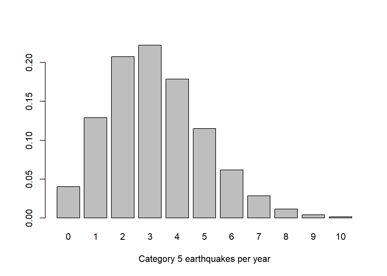
What is the probability that next year has no category 5 earthquakes?

dpois(0, lambda_cat5)

[1] 0.04008846

Of the next 10 years, how many would you expect to have:

No category 5 earthquakes?

dpois(0, lambda_cat5)*10

[1] 0.4008846

Fewer than 2 earthquakes?

ppois(1, lambda_cat5)*10

[1] 1.690397

At least 5?

(1-ppois(4, lambda_cat5))*10

[1] 2.223618