# Not needed if you did this once already
install.packages("tidyverse")tidyverse intro
Unlike in your coursework, real world datasets are often messy. Data often comes from several sources, was collected by different people, entered into a spreadsheet by even different people, and arrives on your computer in multiple arrangements. There may be missing or incorrect values, multiple labels for the same treatment, and many unnecessary columns.
Even with clean datasets, you should spend a good amount of time looking at your data in different ways. This is called Exploratory Data Analysis (EDA). Quick plots and summaries are a great way to identify potential errors and can help you develop an intuitive sense of complex datasets.
The tidyverse is “an opinionated collection of R packages designed for data science” that is commonly used in the R-based data science world. The packages share a common philosophy with a distinct coding grammar and data structures. They work collaboratively to make data science easier, cleaner, and more reproducible.
This is a brief overview – there is much, much more that we will not cover.
What makes a dataset tidy vs. messy?
Within the tidyverse framework, a tidy dataset is one where:
- Each variable is a single column
- Each observation is a single row
- Each type of observational unit is a single table
If you have multiple related spreadsheets, each should have a column with the same name that allows them to be joined or merged appropriately.
Guidelines for data entry
When entering your data, try to keep to the following guidelines:
- Be consistent. Use a single way of entering a variable (Y/N or Yes/No or 0/1).
- Choose good names. Use underscores, camelCase, or SnakeCase instead of spaces. Use short, descriptive names. In R, object names can’t start with numbers or special characters, so try to avoid that in your factor levels as well.
- Write dates as YYYY-MM-DD. This is the global ISO 8601 standard. It sorts well and might keep Excel from mangling your data.
- No empty cells. Enter NA instead.
-
Put just one thing in a cell. Have a column
weight_kgfilled with numbers rather than a column calledweightfilled with values like “5.5 kg”. - Don’t use font color or highlighting as data. Sometimes used to flag values. Instead, create a new column to store the information.
- Save data as plain text files. Proprietary formats like .xlsx can be handy, but plain text (.csv, .txt, .tsv, etc) does not require special software and can be read by anyone on any machine.
Key packages in the tidyverse
There are many packages associated with the tidyverse. We will cover aspects of only a select few:
- tibble: a re-imagining of the dataframe
- dplyr: data manipulation
- tidyr: tidying data
- ggplot2: visualization
- stringr: working with strings
- lubridate: working with dates and date-times
When you install the tidyverse package, all of these are installed (and more).
Review: Piping
As seen in Practical 1, piping helps keep your code legible. The ‘pipe operator’ allows you to string together functions by taking the output of one and sending it as input to the next. Many functions in the tidyverse are designed to work nicely in pipes.
The native R pipe is |> and was introduced in R 4.1.0. Prior to this, piping required the %>% function in the magrittr package, which you may see in help pages or online documentation.
The convenience will become clear as we go.
Tibbles
Tibbles are dataframes, but with a few extra tweaks. See the Tibbles chapter in R for Data Science for a more comprehensive overview.
str(msleep)tibble [83 × 11] (S3: tbl_df/tbl/data.frame)
$ name : chr [1:83] "Cheetah" "Owl monkey" "Mountain beaver" "Greater short-tailed shrew" ...
$ genus : chr [1:83] "Acinonyx" "Aotus" "Aplodontia" "Blarina" ...
$ vore : chr [1:83] "carni" "omni" "herbi" "omni" ...
$ order : chr [1:83] "Carnivora" "Primates" "Rodentia" "Soricomorpha" ...
$ conservation: chr [1:83] "lc" NA "nt" "lc" ...
$ sleep_total : num [1:83] 12.1 17 14.4 14.9 4 14.4 8.7 7 10.1 3 ...
$ sleep_rem : num [1:83] NA 1.8 2.4 2.3 0.7 2.2 1.4 NA 2.9 NA ...
$ sleep_cycle : num [1:83] NA NA NA 0.133 0.667 ...
$ awake : num [1:83] 11.9 7 9.6 9.1 20 9.6 15.3 17 13.9 21 ...
$ brainwt : num [1:83] NA 0.0155 NA 0.00029 0.423 NA NA NA 0.07 0.0982 ...
$ bodywt : num [1:83] 50 0.48 1.35 0.019 600 ...Munging data
It is best to keep your data file in its original form and do all cleaning, filtering, transforming, etc. in R for full transparency and reproducibility. Editing by hand leaves no trail of what you did; mistakes are easy to make but difficult to find.
The dplyr package provides functions for munging data. See the Data Transformation chapter in R for Data Science for a more comprehensive overview.
Key functions:
-
filter()filters rows based on aTRUE/FALSElogical statement -
select()selects columns by name, number, or a tidyselect helper function -
arrange()reorders the tibble according to the column(s) provided -
mutate()creates new columns -
group_by()groups the tibble by the column(s) provided -
summarise()creates summaries, either for the whole tibble or by group
filter()
Use filter() to subset data based on logical statements.
select()
Use select() to select (or exclude) particular columns. There are many selection helpers available, such as starts_with() or ends_with(). Use a negative sign to exclude specified columns.
msleep |>
  select(name, order, starts_with("sleep"))
msleep |>
  select(-conservation)
arrange()
Use arrange() to reorder your data by one or more columns.
mutate()
Use mutate() to create new columns. If you use group_by() first, calculations will be for each group.
summarise()
Use summarise() to create new columns that summarise your data. If you use group_by() first, the summaries will be calculated for each group.
msleep |>
  filter(!is.na(awake)) |>
  summarise(nSpp=n_distinct(name),
            nGenera=n_distinct(genus),
            awake_mean=mean(awake),
            awake_sd=sd(awake))
msleep |>
  filter(!is.na(awake)) |>
  group_by(vore) |>
  summarise(nSpp=n_distinct(name),
            nGenera=n_distinct(genus),
            awake_mean=mean(awake),
            awake_sd=sd(awake))
With the msleep dataset, remove all rows that do not have a conservation status and sort the rows so that they are in alphabetical order by 1) order and 2) genus.
TipView solution
# A tibble: 54 × 11
   name   genus vore  order conservation sleep_total sleep_rem sleep_cycle awake
   <chr>  <chr> <chr> <chr> <chr>              <dbl>     <dbl>       <dbl> <dbl>
 1 Cow    Bos   herbi Arti… domesticated         4         0.7       0.667  20
 2 Roe d… Capr… herbi Arti… lc                   3        NA        NA      21
 3 Goat   Capri herbi Arti… lc                   5.3       0.6      NA      18.7
 4 Giraf… Gira… herbi Arti… cd                   1.9       0.4      NA      22.1
 5 Sheep  Ovis  herbi Arti… domesticated         3.8       0.6      NA      20.2
 6 Pig    Sus   omni  Arti… domesticated         9.1       2.4       0.5    14.9
 7 Cheet… Acin… carni Carn… lc                  12.1      NA        NA      11.9
 8 North… Call… carni Carn… vu                   8.7       1.4       0.383  15.3
 9 Dog    Canis carni Carn… domesticated        10.1       2.9       0.333  13.9
10 Domes… Felis carni Carn… domesticated        12.5       3.2       0.417  11.5
# ℹ 44 more rows
# ℹ 2 more variables: brainwt <dbl>, bodywt <dbl>
In the msleep dataset, how many carnivores sleep more than 8 hours? What proportion of carnivore species is this?
TipView solution
Reshaping data
The tidyr package has many functions for tidying your datasets. We will cover just two that tend to be particularly useful.
Key functions:
-
pivot_longer()takes a series of columns and stacks them into one -
pivot_wider()takes a single column and spreads it into several
pivot_longer()
Use pivot_longer() to stack columns (cols=), specifying new columns to store the original column values (values_to=) and original column names (names_to=).
msleep |>
  select(name, brainwt, bodywt) |>
  pivot_longer(cols=c("brainwt", "bodywt"),
               names_to="structure",
               values_to="weight")
pivot_wider()
Use pivot_wider() to spread the values from single column (values_from=) into several based on a categorical column (names_from=).
iris |>
  group_by(Species) |>
  mutate(Plant_id=row_number()) |>
  ungroup() |>
  select(Plant_id, Species, Petal.Width) |>
  pivot_wider(names_from="Species", values_from="Petal.Width")
With the iris dataset, select the columns for species, petal width, and sepal width, then transform it to be longer with columns Species, FlowerPart, and Width.
TipView solution
Code (bonus)
iris |>
  select(Species, Petal.Width, Sepal.Width) |>
  pivot_longer(c("Petal.Width", "Sepal.Width"),
               names_to="FlowerPart",
               values_to="Width")
# A tibble: 300 × 3
Species FlowerPart Width
<fct> <chr> <dbl>
1 setosa Petal.Width 0.2
2 setosa Sepal.Width 3.5
3 setosa Petal.Width 0.2
4 setosa Sepal.Width 3
5 setosa Petal.Width 0.2
6 setosa Sepal.Width 3.2
7 setosa Petal.Width 0.2
8 setosa Sepal.Width 3.1
9 setosa Petal.Width 0.2
10 setosa Sepal.Width 3.6
# ℹ 290 more rowsWith the msleep dataset, calculate the mean awake time for each feeding type (vore) and then transform it so that there is a single row and a column for each feeding type.
TipView solution
Code (bonus)
msleep |>
  group_by(vore) |>
  summarise(mean=mean(awake)) |>
  pivot_wider(names_from="vore", values_from="mean")
# A tibble: 1 × 5
carni herbi insecti omni `NA`
<dbl> <dbl> <dbl> <dbl> <dbl>
1 13.6 14.5 9.06 13.1 13.8ggplot2
The ggplot2 package is fantastic for exploratory data analysis, as well as creating polished plots for final presentation. See the ‘reference’ tab on the package website for all plotting functions, and the Exploratory Data Analysis chapter and the Graphics for Communication chapter in R for Data Science for many examples and much more information.
Key functions:
-
ggplot()initializes a plot object; always used first, followed by+ -
geom_*()plot elements (e.g.,geom_point(),geom_line(), etc) -
geom_smooth()calculates and plots a trend line -
scale_colour_*()specifies a custom colour palette -
scale_fill_*()specifies a custom fill palette -
scale_x/y_*()specifies a custom x or y axis -
labs()adds labels (x, y, title, subtitle) -
facet_wrap(),facet_grid()partition data into panels by the specified variable(s)
Scatter plots
# scatter plot
msleep |>
  ggplot(aes(brainwt, bodywt)) +
  geom_point()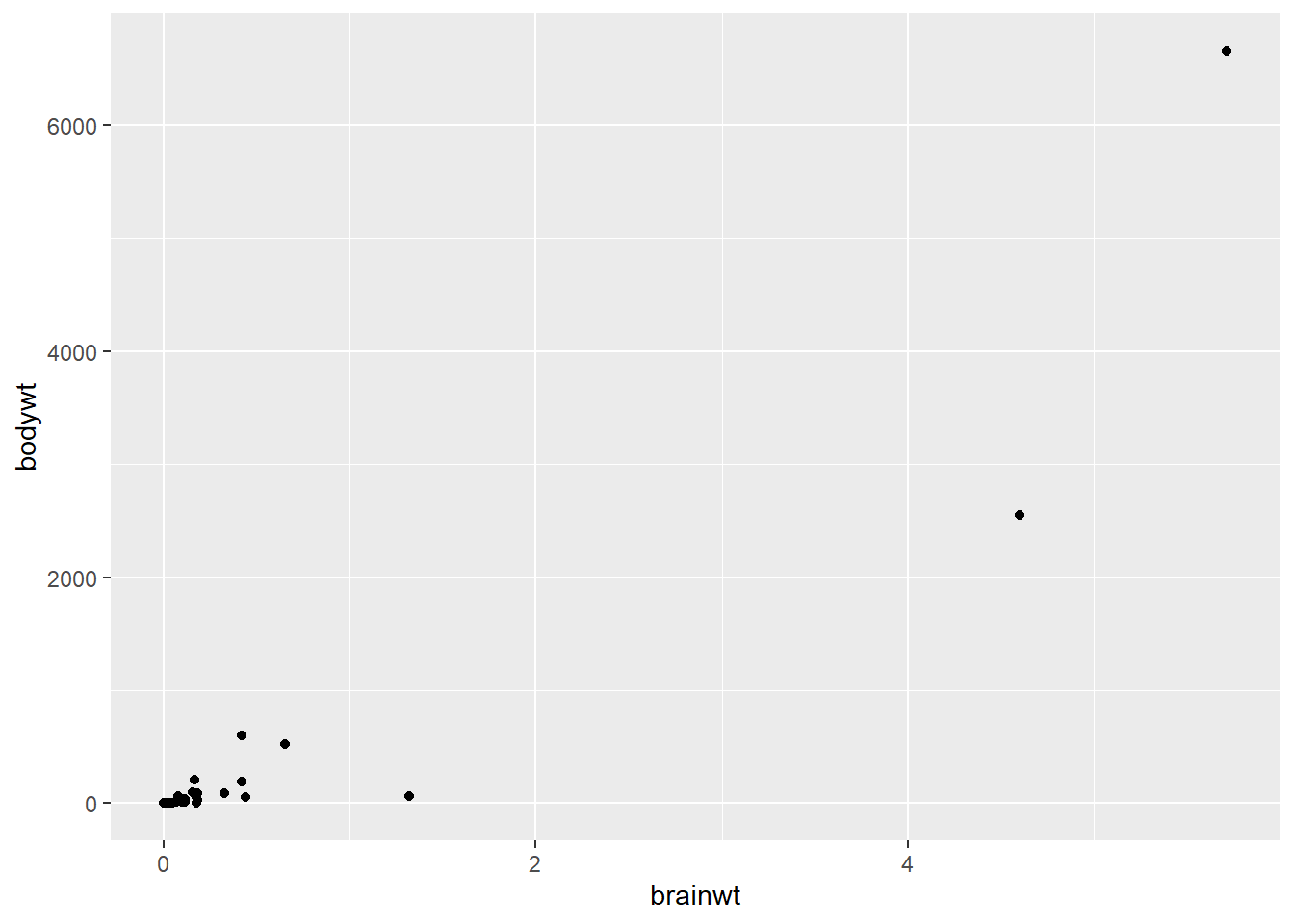
msleep |>
  ggplot(aes(brainwt, bodywt)) +
  geom_point() +
  scale_x_log10("Brain weight (kg)") +
  scale_y_log10("Body weight (kg)")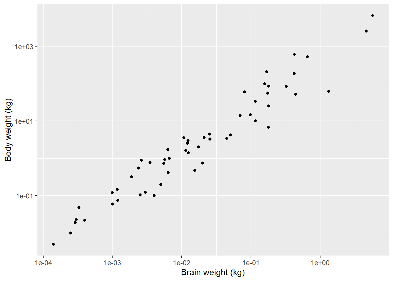
Histograms, etc
# histogram
msleep |>
  ggplot(aes(sleep_cycle)) +
  geom_histogram()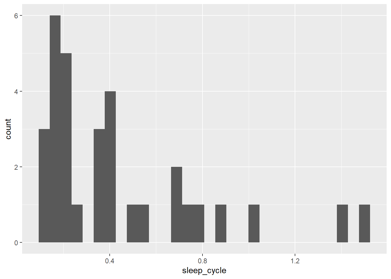
# density plot
msleep |>
  ggplot(aes(sleep_cycle)) +
  geom_density()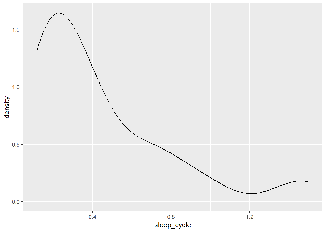
# box plot
msleep |>
  ggplot(aes(vore, sleep_cycle)) +
  geom_boxplot()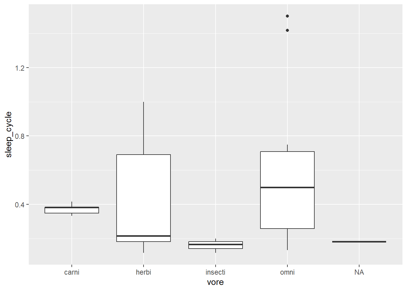
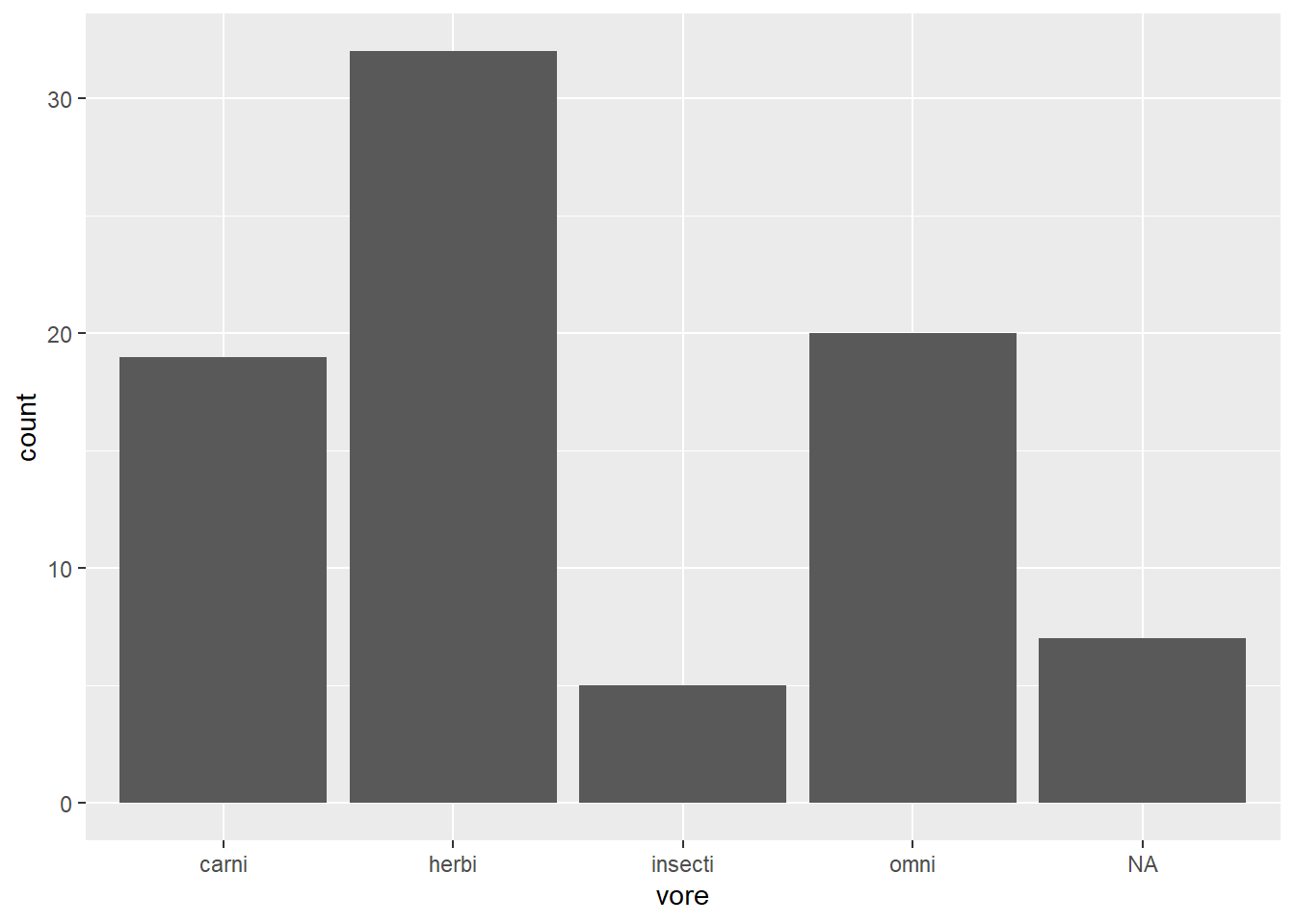
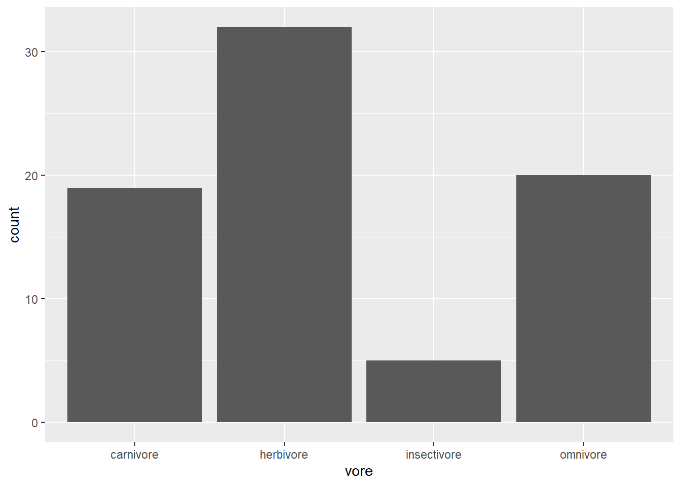
Trend lines
# scatter plot with group-level trend lines
iris |>
  ggplot(aes(Sepal.Length, Petal.Length, colour=Species)) +
  geom_point() +
  geom_smooth(method="lm")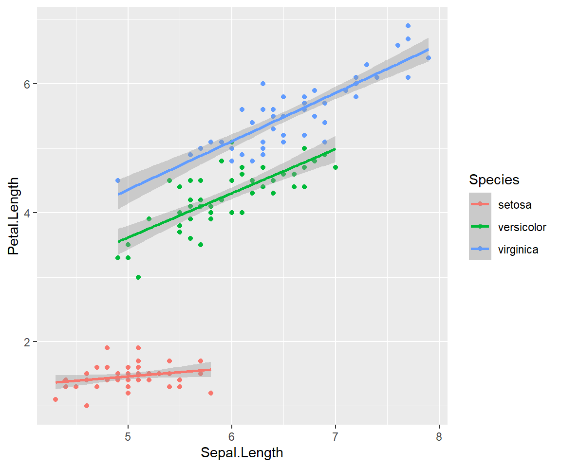
# scatter plot with global trend line
iris |>
  ggplot(aes(Sepal.Length, Petal.Length)) +
  geom_point(aes(colour=Species)) +
  geom_smooth(method="lm")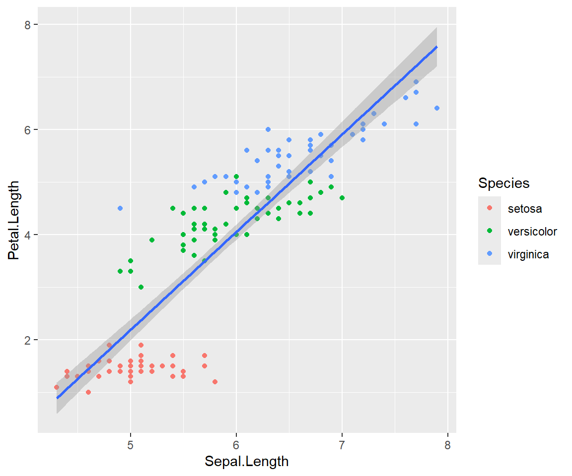
# scatter plot with global and group-level trend lines
iris |>
  ggplot(aes(Sepal.Length, Petal.Length)) +
  geom_point(aes(colour=Species)) +
  geom_smooth(method="lm", colour="black") +
  geom_smooth(aes(colour=Species), method="lm") +
  labs(x="Sepal length (cm)",
       y="Petal length (cm)",
       title="Global vs. local aesthetics",
       subtitle="Built-in data set `iris`")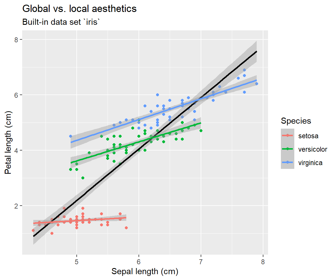
Bells and whistles
There are endless options for making your plot just as you like. Colour can be specified with functions taking the form scale_colour_*() or scale_fill_*() (e.g., see ?scale_fill_manual). The details of the plot elements can be specified within the geom_*() functions (e.g., see ?geom_point). Panels can be added using facet_wrap(~col_A) or facet_grid(col_A ~ col_B). Axes also have their own functions (e.g., see ?scale_x_continuous). Plots also have themes, which can be specified manually using theme() or by adding pre-specified themes like theme_classic() or theme_bw().
# specify a colour scale with species as panels
iris |>
  mutate(Sepal.Area=Sepal.Length*Sepal.Width) |>
  ggplot(aes(Petal.Length, Petal.Width, colour=Sepal.Width)) +
  geom_point() +
  scale_colour_viridis_c() +
  facet_wrap(~Species)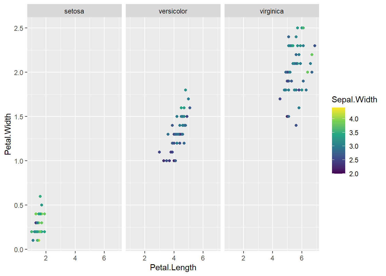
# use arguments within facet_wrap() to have 1 column of panels
iris |>
  mutate(Sepal.Area=Sepal.Length*Sepal.Width) |>
  ggplot(aes(Petal.Length, Petal.Width, colour=Sepal.Width)) +
  geom_point() +
  scale_colour_viridis_c() +
  facet_wrap(~Species, ncol=1)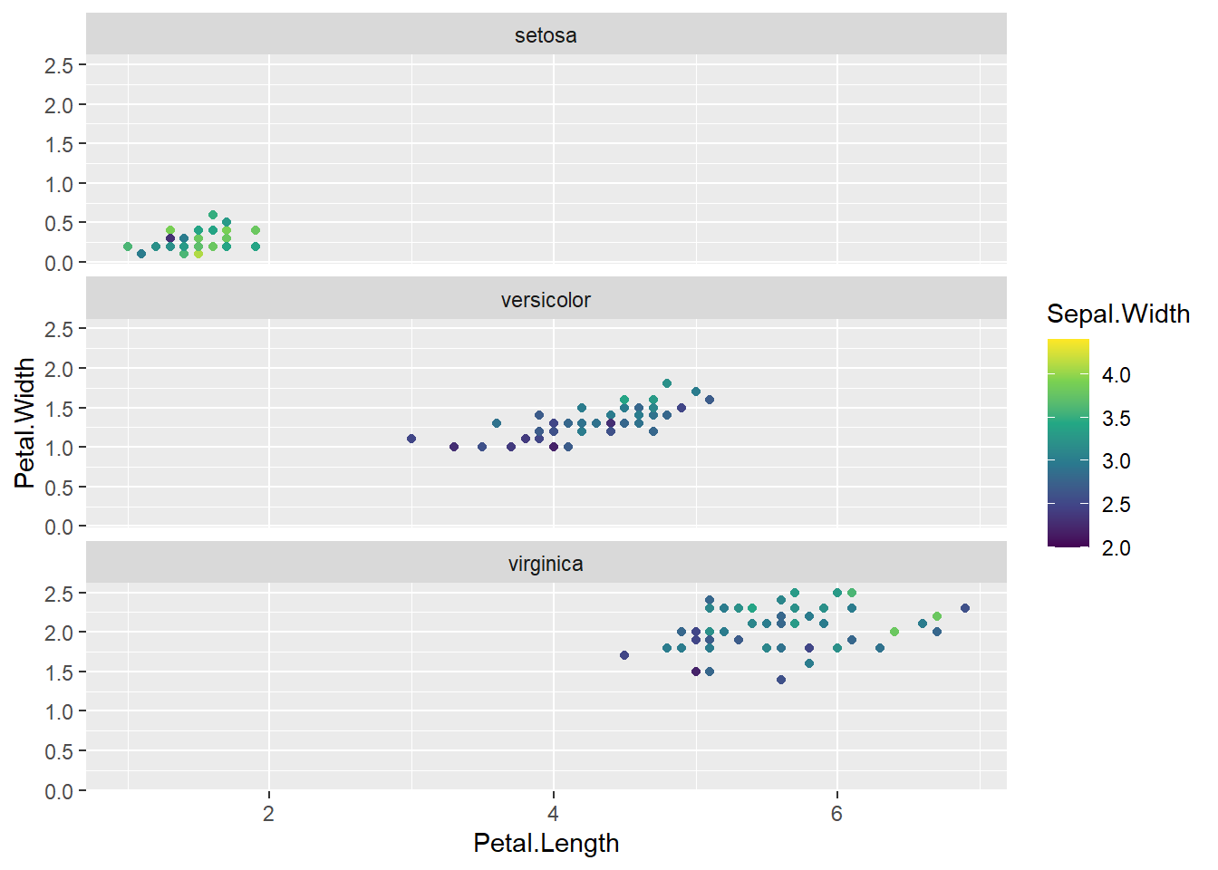
# specify geom_bar() arguments, add a fill, labels, theme, etc
msleep |>
  filter(!is.na(vore) & !is.na(conservation)) |>
  mutate(vore=paste0(vore, "vore"),
         conservation=factor(conservation,
                             levels=c("domesticated", "lc", "cd", "nt", "vu", "en"))) |>
  ggplot(aes(vore, fill=conservation)) +
  geom_bar(position="fill", colour="grey30") +
  scale_fill_brewer("Conservation\nstatus", type="seq", palette="Reds") +
  labs(y="Proportion of species",
       title="Conservation status in the msleep dataset") +
  theme_classic() +
  theme(axis.title.x=element_blank())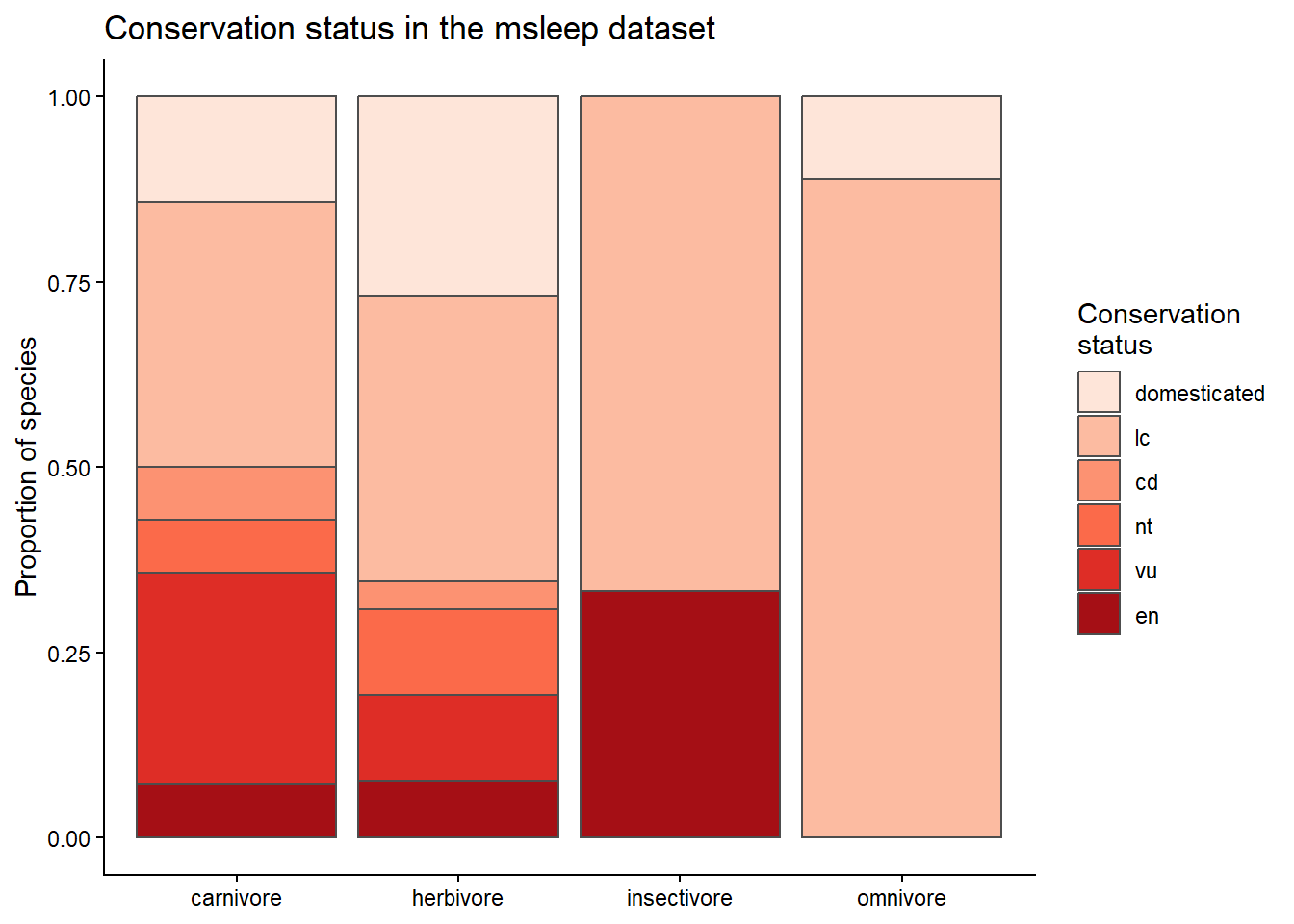
These can all be combined in any way you can imagine.
Explore the msleep dataset further using ggplot. For example, is there an association between sleep and brain weight as a proportion of body weight? Does this depend on feeding strategy? Do larger species spend more time sleeping?
Create a histogram of body weight with each feeding strategy in a different panel. Try transforming the x-axis to log-10 scale. Adjust the number of bins in the histograms and change the fill and colour of the bars. Add axis labels.
TipView solution
Code (bonus)
msleep |>
  ggplot(aes(bodywt)) +
  geom_histogram(bins=12, colour="black", fill="steelblue") +
  scale_x_log10() +
  facet_wrap(~vore) +
  labs(x="Body weight (kg)", y="Number of species")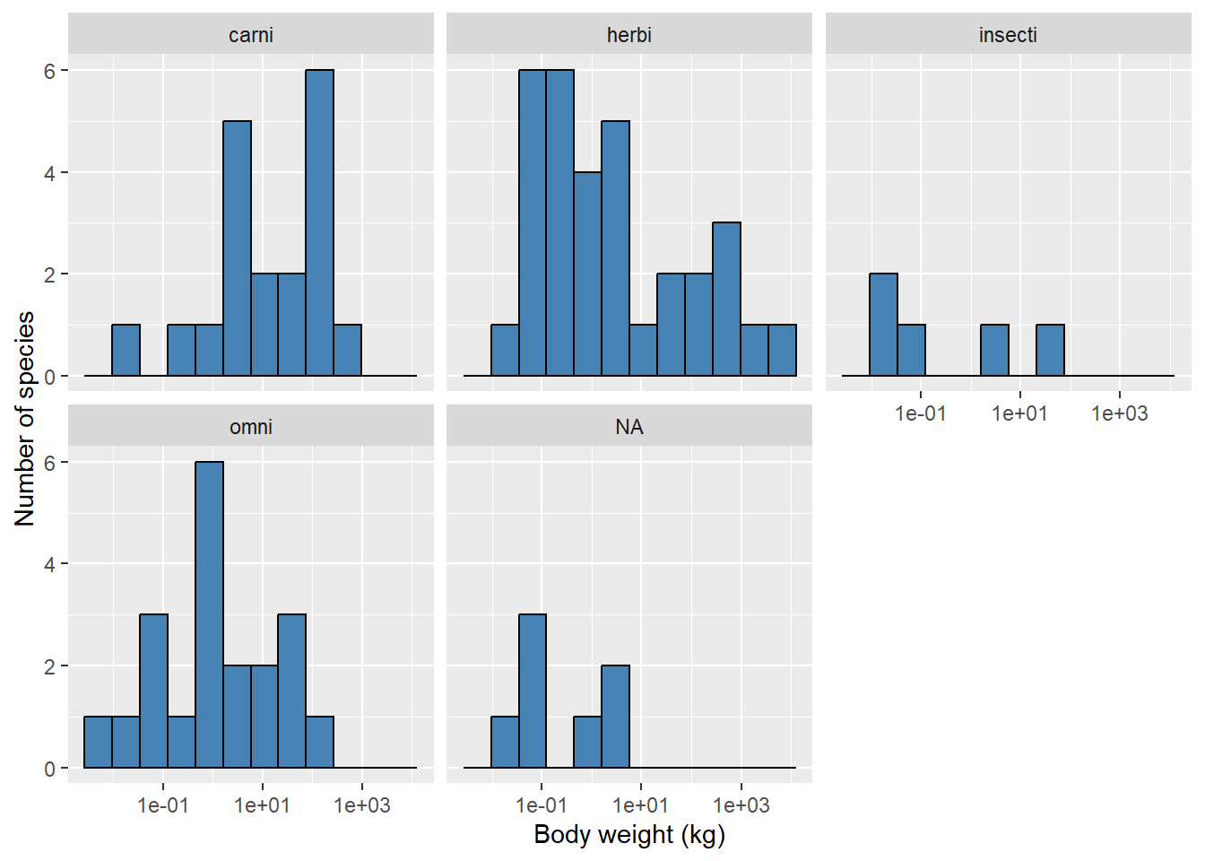
Working with strings
The stringr package has many convenient functions for working with strings (text). They generally follow the naming form of str_verb(). See the Strings chapter in R for Data Science for a more comprehensive overview.
Key functions:
-
str_remove()removes a pattern from each element in the vector -
str_replace()replaces a pattern from each element in the vector -
str_sub()extracts a subset of characters from each element in the vector -
str_split()splits each element in the vector based on a pattern
TipView examples
str_remove()
msleep |>
  select(name, genus) |>
  mutate(nameNoSpace=str_remove(name, " "))
msleep |>
  select(name, genus) |>
  mutate(nameNoSpace=str_remove_all(name, " "))
str_replace()
msleep |>
  select(name, genus) |>
  mutate(nameNoSpace=str_replace(name, " ", "_"))
# A tibble: 83 × 3
name genus nameNoSpace
<chr> <chr> <chr>
1 Cheetah Acinonyx Cheetah
2 Owl monkey Aotus Owl_monkey
3 Mountain beaver Aplodontia Mountain_beaver
4 Greater short-tailed shrew Blarina Greater_short-tailed shrew
5 Cow Bos Cow
6 Three-toed sloth Bradypus Three-toed_sloth
7 Northern fur seal Callorhinus Northern_fur seal
8 Vesper mouse Calomys Vesper_mouse
9 Dog Canis Dog
10 Roe deer Capreolus Roe_deer
# ℹ 73 more rowsmsleep |>
select(name, genus) |>
mutate(nameNoSpace=str_replace_all(name, " ", "_"))# A tibble: 83 × 3
name genus nameNoSpace
<chr> <chr> <chr>
1 Cheetah Acinonyx Cheetah
2 Owl monkey Aotus Owl_monkey
3 Mountain beaver Aplodontia Mountain_beaver
4 Greater short-tailed shrew Blarina Greater_short-tailed_shrew
5 Cow Bos Cow
6 Three-toed sloth Bradypus Three-toed_sloth
7 Northern fur seal Callorhinus Northern_fur_seal
8 Vesper mouse Calomys Vesper_mouse
9 Dog Canis Dog
10 Roe deer Capreolus Roe_deer
# ℹ 73 more rowsstr_sub()
# A tibble: 83 × 4
   name                       genus       order        order_abbr
   <chr>                      <chr>       <chr>        <chr>
 1 Cheetah                    Acinonyx    Carnivora    Carn
 2 Owl monkey                 Aotus       Primates     Prim
 3 Mountain beaver            Aplodontia  Rodentia     Rode
 4 Greater short-tailed shrew Blarina     Soricomorpha Sori
 5 Cow                        Bos         Artiodactyla Arti
 6 Three-toed sloth           Bradypus    Pilosa       Pilo
 7 Northern fur seal          Callorhinus Carnivora    Carn
 8 Vesper mouse               Calomys     Rodentia     Rode
 9 Dog                        Canis       Carnivora    Carn
10 Roe deer                   Capreolus   Artiodactyla Arti
# ℹ 73 more rows
str_split()
# A tibble: 83 × 4
   name                       genus       order        nameSplit
   <chr>                      <chr>       <chr>        <list>
 1 Cheetah                    Acinonyx    Carnivora    <chr [1]>
 2 Owl monkey                 Aotus       Primates     <chr [2]>
 3 Mountain beaver            Aplodontia  Rodentia     <chr [2]>
 4 Greater short-tailed shrew Blarina     Soricomorpha <chr [3]>
 5 Cow                        Bos         Artiodactyla <chr [1]>
 6 Three-toed sloth           Bradypus    Pilosa       <chr [2]>
 7 Northern fur seal          Callorhinus Carnivora    <chr [3]>
 8 Vesper mouse               Calomys     Rodentia     <chr [2]>
 9 Dog                        Canis       Carnivora    <chr [1]>
10 Roe deer                   Capreolus   Artiodactyla <chr [2]>
# ℹ 73 more rows[[1]]
[1] "Cheetah"
[[2]]
[1] "Owl" "monkey"
[[3]]
[1] "Mountain" "beaver"
[[4]]
[1] "Greater" "short-tailed" "shrew"
[[5]]
[1] "Cow"
[[6]]
[1] "Three-toed" "sloth" str_split_fixed(msleep$name, " ", 3) |> head() [,1] [,2] [,3]
[1,] "Cheetah" "" ""
[2,] "Owl" "monkey" ""
[3,] "Mountain" "beaver" ""
[4,] "Greater" "short-tailed" "shrew"
[5,] "Cow" "" ""
[6,] "Three-toed" "sloth" "" str_split_fixed(msleep$name, " ", 3)[,1] [1] "Cheetah" "Owl" "Mountain" "Greater"
[5] "Cow" "Three-toed" "Northern" "Vesper"
[9] "Dog" "Roe" "Goat" "Guinea"
[13] "Grivet" "Chinchilla" "Star-nosed" "African"
[17] "Lesser" "Long-nosed" "Tree" "North"
[21] "Asian" "Big" "Horse" "Donkey"
[25] "European" "Patas" "Western" "Domestic"
[29] "Galago" "Giraffe" "Pilot" "Gray"
[33] "Gray" "Human" "Mongoose" "African"
[37] "Thick-tailed" "Macaque" "Mongolian" "Golden"
[41] "Vole" "House" "Little" "Round-tailed"
[45] "Slow" "Degu" "Northern" "Rabbit"
[49] "Sheep" "Chimpanzee" "Tiger" "Jaguar"
[53] "Lion" "Baboon" "Desert" "Potto"
[57] "Deer" "Phalanger" "Caspian" "Common"
[61] "Potoroo" "Giant" "Rock" "Laboratory"
[65] "African" "Squirrel" "Eastern" "Cotton"
[69] "Mole" "Arctic" "Thirteen-lined" "Golden-mantled"
[73] "Musk" "Pig" "Short-nosed" "Eastern"
[77] "Brazilian" "Tenrec" "Tree" "Bottle-nosed"
[81] "Genet" "Arctic" "Red" Working with dates
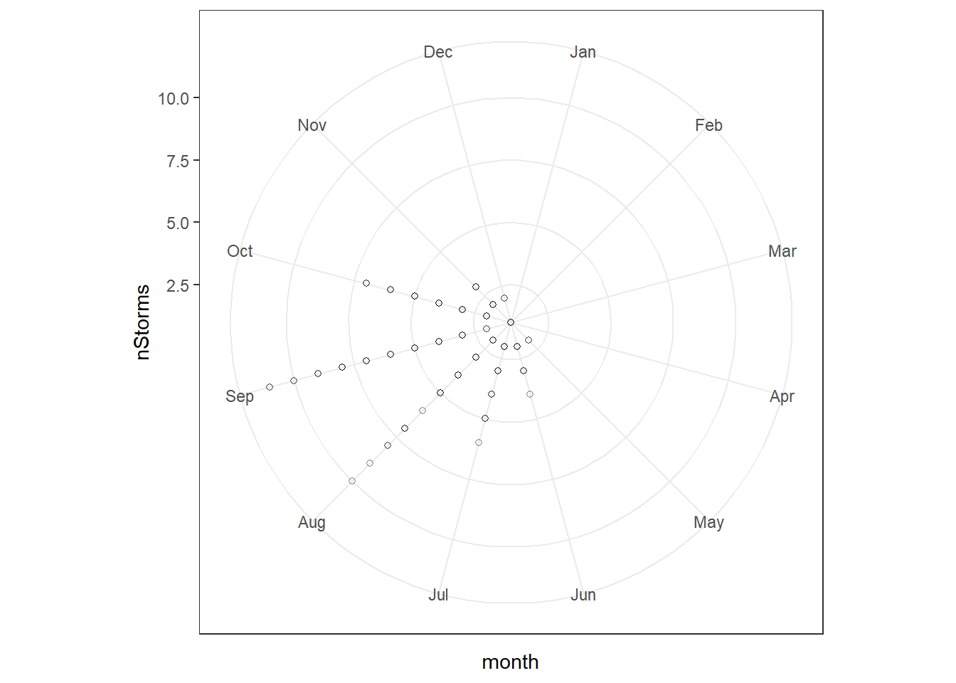
Date-time data are notoriously prickly, and R is no exception. The lubridate package makes them much less so. See the Dates and Times chapter in R for Data Science for a more comprehensive overview.
Key functions:
-
ymd(),mdy(),dmy()convert a string with year, month, and day into a date -
ymd_hms()converts a string to a date-time, including hour, minutes, and seconds -
year(),month(),mday(),yday(),week()extract the corresponding component - adding and subtracting work intuitively
- plotting with ggplot2 is straightforward
TipView examples
str(storms)tibble [20,778 × 13] (S3: tbl_df/tbl/data.frame)
$ name : chr [1:20778] "Amy" "Amy" "Amy" "Amy" ...
$ year : num [1:20778] 1975 1975 1975 1975 1975 ...
$ month : num [1:20778] 6 6 6 6 6 6 6 6 6 6 ...
$ day : int [1:20778] 27 27 27 27 28 28 28 28 29 29 ...
$ hour : num [1:20778] 0 6 12 18 0 6 12 18 0 6 ...
$ lat : num [1:20778] 27.5 28.5 29.5 30.5 31.5 32.4 33.3 34 34.4 34 ...
$ long : num [1:20778] -79 -79 -79 -79 -78.8 -78.7 -78 -77 -75.8 -74.8 ...
$ status : Factor w/ 9 levels "disturbance",..: 7 7 7 7 7 7 7 7 8 8 ...
$ category : num [1:20778] NA NA NA NA NA NA NA NA NA NA ...
$ wind : int [1:20778] 25 25 25 25 25 25 25 30 35 40 ...
$ pressure : int [1:20778] 1013 1013 1013 1013 1012 1012 1011 1006 1004 1002 ...
$ tropicalstorm_force_diameter: int [1:20778] NA NA NA NA NA NA NA NA NA NA ...
$ hurricane_force_diameter : int [1:20778] NA NA NA NA NA NA NA NA NA NA ...tibble [20,778 × 6] (S3: tbl_df/tbl/data.frame)
$ name: chr [1:20778] "AL011993" "AL011993" "AL011993" "AL011993" ...
$ date: Date[1:20778], format: "1993-05-31" "1993-05-31" ...
$ time: POSIXct[1:20778], format: "1993-05-31 12:00:00" "1993-05-31 18:00:00" ...
$ long: num [1:20778] -84 -82 -80.3 -79 -77.5 -75.8 -74 -71.8 -69.9 -67.8 ...
$ lat : num [1:20778] 21.5 22.3 23.2 24.5 25.4 26.1 26.7 27.8 28.4 28.5 ...
$ wind: int [1:20778] 25 25 25 25 30 30 30 30 35 35 ...storms_df |>
mutate(month=month(date, label=T)) |>
ggplot(aes(month, wind)) +
geom_boxplot() +
scale_x_discrete(limits=month.abb)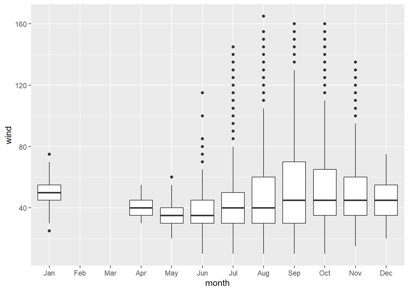
storms_df |>
  mutate(week=week(date),
         year=year(date)) |>
  group_by(year, week) |>
  summarise(nStorms=n_distinct(name),
            mnWind=mean(wind)) |>
  ungroup() |>
  pivot_longer(c("nStorms", "mnWind"),
               names_to="metric", values_to="value") |>
  ggplot(aes(week, value, group=year)) +
  geom_jitter(alpha=0.5, shape=1, width=0, height=0.25) +
  coord_polar() +
  theme_bw() +
  facet_wrap(~metric, scales="free_y")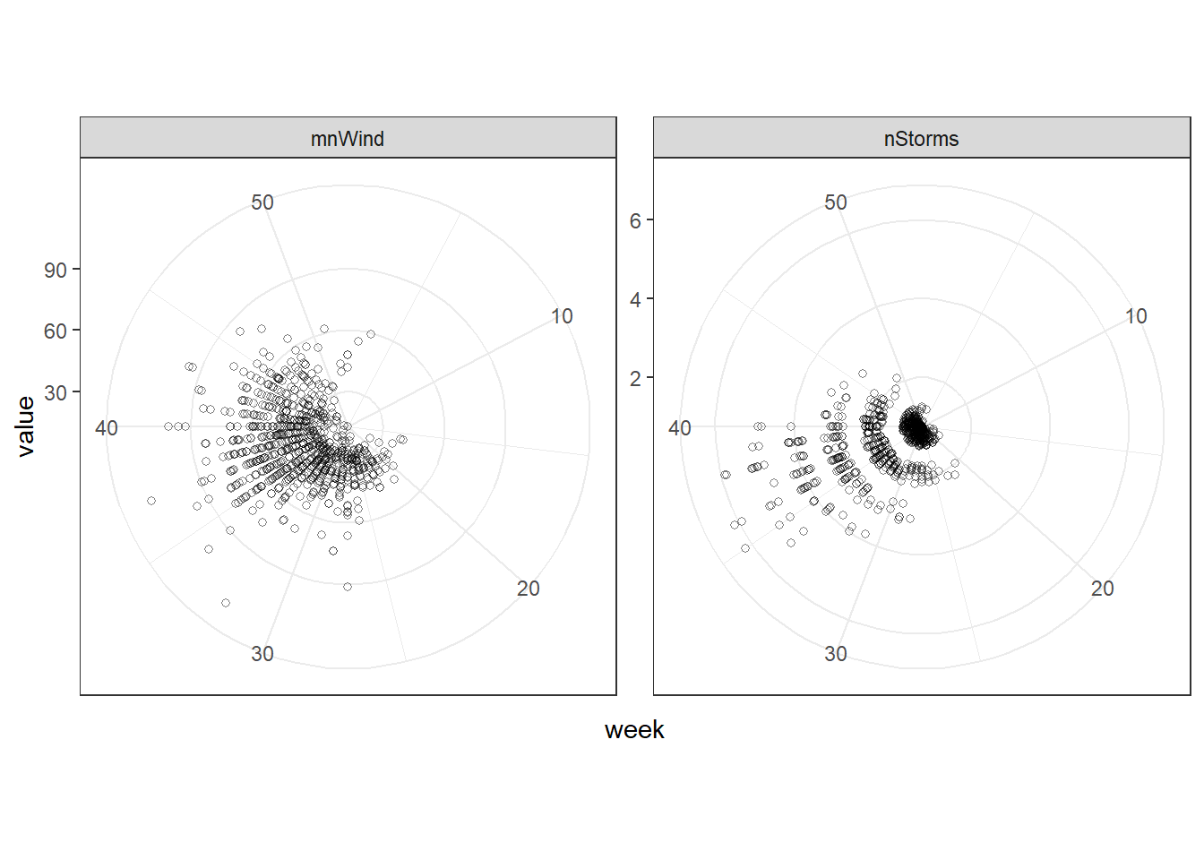
storms_df |>
  mutate(month=month(date, label=T),
         year=year(date)) |>
  group_by(year, month) |>
  summarise(nStorms=n_distinct(name),
            mnWind=mean(wind)) |>
  ggplot(aes(month, mnWind, group=year)) +
  geom_point(alpha=0.5, shape=1) +
  scale_x_discrete(limits=month.abb) +
  coord_polar() +
  theme_bw()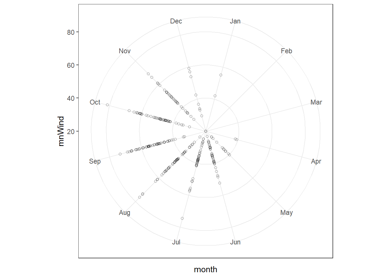
storms_df |>
  mutate(month=month(date, label=T),
         year=year(date)) |>
  group_by(year, month) |>
  summarise(nStorms=n_distinct(name),
            mnWind=mean(wind)) |>
  ggplot(aes(month, nStorms, group=year)) +
  geom_point(alpha=0.5, shape=1) +
  scale_x_discrete(limits=month.abb) +
  coord_polar() +
  theme_bw()