Problem Set 1

Please render this file to .html and submit via Brightspace.

library(tidyverse); theme_set(theme_classic())
library(readxl)
set.seed(2026)

R Basics

Data types

Create a vector called site_num with the values 1 through 10.

Three methods which create identical vectors

site_num <- 1:10
site_num <- seq(1, 10, by=1)
site_num <- c(1, 2, 3, 4, 5, 6, 7, 8, 9, 10)

Create a matrix called pop_abund with the values 101 through 120, with 2 columns and 10 rows.

Matrix creation

pop_abund <- matrix(101:120, ncol=2, nrow=10)

Create a copy of the dataframe iris (already available as iris) and name it iris_df. View the column names and create a new column called Petal.Area, calculated as Petal.Width times Petal.Length.

Make iris_df

iris_df <- iris

View column names (method 1)

names(iris_df)

[1] "Sepal.Length" "Sepal.Width"  "Petal.Length" "Petal.Width"  "Species"

View column names (method 2)

str(iris_df)

'data.frame':   150 obs. of  5 variables:
 $ Sepal.Length: num  5.1 4.9 4.7 4.6 5 5.4 4.6 5 4.4 4.9 ...
 $ Sepal.Width : num  3.5 3 3.2 3.1 3.6 3.9 3.4 3.4 2.9 3.1 ...
 $ Petal.Length: num  1.4 1.4 1.3 1.5 1.4 1.7 1.4 1.5 1.4 1.5 ...
 $ Petal.Width : num  0.2 0.2 0.2 0.2 0.2 0.4 0.3 0.2 0.2 0.1 ...
 $ Species     : Factor w/ 3 levels "setosa","versicolor",..: 1 1 1 1 1 1 1 1 1 1 ...

View column names (method 3)

glimpse(iris_df)

Rows: 150
Columns: 5
$ Sepal.Length <dbl> 5.1, 4.9, 4.7, 4.6, 5.0, 5.4, 4.6, 5.0, 4.4, 4.9, 5.4, 4.…
$ Sepal.Width  <dbl> 3.5, 3.0, 3.2, 3.1, 3.6, 3.9, 3.4, 3.4, 2.9, 3.1, 3.7, 3.…
$ Petal.Length <dbl> 1.4, 1.4, 1.3, 1.5, 1.4, 1.7, 1.4, 1.5, 1.4, 1.5, 1.5, 1.…
$ Petal.Width  <dbl> 0.2, 0.2, 0.2, 0.2, 0.2, 0.4, 0.3, 0.2, 0.2, 0.1, 0.2, 0.…
$ Species      <fct> setosa, setosa, setosa, setosa, setosa, setosa, setosa, s…

Create a new column (method 1)

iris_df$Petal.Area <- iris_df$Petal.Width * iris_df$Petal.Length

Create a new column (method 2)

iris_df <- iris_df |>
  mutate(Petal.Area=Petal.Width*Petal.Length)

Data munging

The SmoltWeights sheet from H2SMS_practicalData.xlsx contains the weight in grams (column weight_g) from a sample of 34 wild salmon smolts (column fish_id) during their out-migration from a river to the ocean. Load the dataset and perform basic summaries (range, mean, median, number of missing values for each column). Identify (using code) which fish are missing values for weight_g.

Load and check data

smolt_df <- read_xlsx("data/H2SMS_practicalData.xlsx", sheet="SmoltWeights")
str(smolt_df)

tibble [34 × 2] (S3: tbl_df/tbl/data.frame)
 $ fish_id : num [1:34] 1 2 3 4 5 6 7 8 9 10 ...
 $ weight_g: num [1:34] 44.2 40.2 39.7 36 40.9 33.8 51.2 41.1 36.7 37.2 ...

Load and check data

summary(smolt_df)

    fish_id         weight_g    
 Min.   : 1.00   Min.   :26.60  
 1st Qu.: 9.25   1st Qu.:36.00  
 Median :17.50   Median :39.70  
 Mean   :17.50   Mean   :40.17  
 3rd Qu.:25.75   3rd Qu.:46.10  
 Max.   :34.00   Max.   :51.20  
                 NA's   :1

There are many ways to identify the row with missing data.

Method 1: Identify the row number

which(is.na(smolt_df$weight_g))

[1] 12

Method 2: Extract the row from the data.frame

smolt_df[is.na(smolt_df$weight_g),] # gives the row from the data.frame

# A tibble: 1 × 2
  fish_id weight_g
    <dbl>    <dbl>
1      12       NA

Method 3: Filter the data.frame

smolt_df |>
  filter(is.na(weight_g))

# A tibble: 1 × 2
  fish_id weight_g
    <dbl>    <dbl>
1      12       NA

Create a new column called weight_lb that gives the weights in pounds, where 1 kg = 2.205 lb.

Calculate new column

smolt_df$weight_lb <- smolt_df$weight_g / 1000 * 2.205

What proportion of fish weigh less than 0.2 lb? How many fish is this?

Proportion

mean(smolt_df$weight_lb < 0.2, na.rm=T)

[1] 1

Number

sum(smolt_df$weight_lb < 0.2, na.rm=T)

[1] 33

Create a new data.frame called large_df that contains only the fish as large or larger than the median weight and excludes rows with missing weights.

# A tibble: 17 × 3
   fish_id weight_g weight_lb
     <dbl>    <dbl>     <dbl>
 1       1     44.2    0.0975
 2       2     40.2    0.0886
 3       3     39.7    0.0875
 4       5     40.9    0.0902
 5       7     51.2    0.113 
 6       8     41.1    0.0906
 7      17     46.7    0.103 
 8      20     46.1    0.102 
 9      21     50.9    0.112 
10      22     45.7    0.101 
11      23     46.8    0.103 
12      24     50.5    0.111 
13      25     46.7    0.103 
14      29     41.8    0.0922
15      32     41.5    0.0915
16      33     47.3    0.104 
17      34     48.9    0.108

Using base R functions

smolt_median <- median(smolt_df$weight_g, na.rm=T)
large_df <- smolt_df[smolt_df$weight_g >= smolt_median & !is.na(smolt_df$weight_g), ]

Using tidyverse functions

large_df <- smolt_df |>
  drop_na(weight_g) |>
  filter(weight_g >= median(weight_g))

Create a new data.frame called extreme_df that contains only fish more than 1.5 standard deviations greater than the mean and excludes rows with missing weights.

# A tibble: 3 × 3
  fish_id weight_g weight_lb
    <dbl>    <dbl>     <dbl>
1       7     51.2     0.113
2      21     50.9     0.112
3      24     50.5     0.111

Using base R functions

smolt_mean <- mean(smolt_df$weight_g, na.rm=T)
smolt_sd <- sd(smolt_df$weight_g, na.rm=T)
rows_to_keep <- !is.na(smolt_df$weight_g) &
                         (smolt_df$weight_g > smolt_mean + 1.5*smolt_sd)
extreme_df <- smolt_df[rows_to_keep, ]

Using tidyverse functions

extreme_df <- smolt_df |>
  drop_na(weight_g) |>
  filter(weight_g > mean(weight_g) + 1.5*sd(weight_g))

Plotting

Histograms

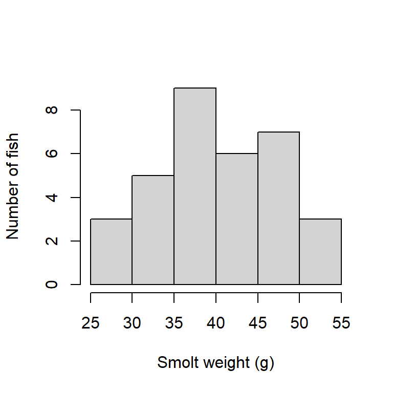
Create a histogram of the smolt weights, labelling the axes and omitting a plot title. Add a figure legend using #| fig-cap: "..." in the quarto document code block. Add #| label: fig-smoltHist, and then in text below, reference the figure by typing @fig-smoltHist.

When rendered, @fig-smoltHist in the text is automatically replaced by “Figure 1”, with figure numbers updated automatically. Adding a legend with #| fig-cap: "..." in your code block will automatically give that figure a number, making your life easier.

The label must start with fig- for this to work.

Note that you cannot re-use the same label.

Here is some text referencing Figure 1 by using the label I’ve used in the code chunk (@fig-smoltHist).

Code chunk

```{r}
#| code-fold: true
#| code-summary: "Code chunk"
#| label: fig-smoltHist
#| fig-cap: "Histogram of smolt weights."
#| fig-width: 4
#| fig-height: 4

hist(smolt_df$weight_g, 
     main=NULL, 
     xlab="Smolt weight (g)",
     ylab="Number of fish")
```

Line plots

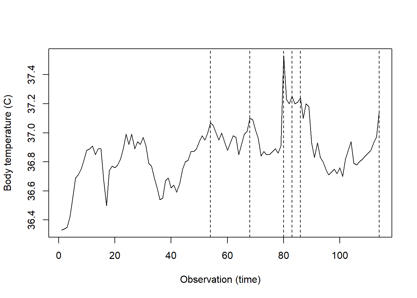
The dataset beaver1 is available in R, giving the body temperature through time of a female beaver (Castor canadensis), with observations every 10 minutes.

str(beaver1)

'data.frame':   114 obs. of  4 variables:
 $ day  : num  346 346 346 346 346 346 346 346 346 346 ...
 $ time : num  840 850 900 910 920 930 940 950 1000 1010 ...
 $ temp : num  36.3 36.3 36.4 36.4 36.5 ...
 $ activ: num  0 0 0 0 0 0 0 0 0 0 ...

Debug the following code so that it produces a line plot of body temperature by observation id. Note that time is given in the form 0330 for 3:30am (?beaver1). The obs_id column thus gives the ordered observations from first to last.

As an added challenge, add vertical dashed lines indicating when the beaver was active.

Set #| eval: true to run the code when you click Render. If you’ve successfully debugged, you should then see your plot.

beaver_df <- beaver1
beaver_df$obs_id <- 1:nrow(beaver_df)
plot(obs_id ~ Temp, 
     data=beaver_df, 
     type="p", 
     xLab="Observation (time)",
     ylab="Body temperature (C)")

Original:

beaver_df <- beaver1
beaver_df$obs_id <- 1:nrow(beaver_df)
plot(obs_id ~ Temp, # Order is flipped (y ~ x) and `temp` should be lower case
     data=beaver_df, 
     type="p", # Should be "l" (line) or "b" (line with points) 
     xLab="Observation (time)", # typo: lower case l
     ylab="Body temperature (C)")

Corrected:

beaver_df <- beaver1
beaver_df$obs_id <- 1:nrow(beaver_df)
plot(temp ~ obs_id, data=beaver_df, type="l", 
     xlab="Observation (time)",
     ylab="Body temperature (C)")
# ?abline
abline(v=beaver_df$obs_id[beaver_df$activ==1], lty=2)

Boxplots

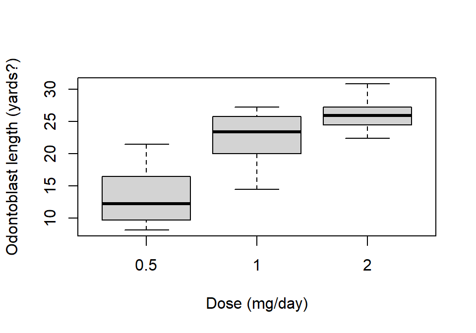
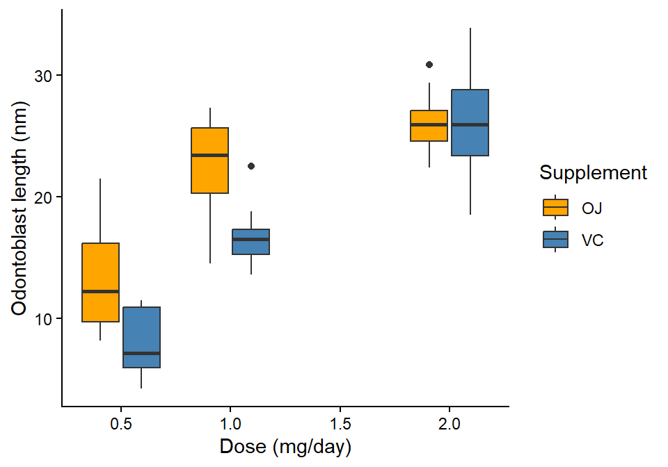
The dataset ToothGrowth is available in R, giving the length (len) of tooth-growth cells (odontoblasts) in 60 guinea pigs under different vitamin C regimes (supp: OJ=orange juice, VC=ascorbic acid; dose: 0.5, 1, 2 mg/day). Create a boxplot of the length by dose for only the guinea pigs receiving orange juice. Write a figure caption and add a label as above.

Using base R

```{r}
#| code-fold: true
#| code-summary: "Using base R"
#| label: fig-OJ_lenByDose
#| fig-cap: "Odontoblast length by dosage in guinea pigs receiving orange juice."
#| fig-width: 5
#| fig-height: 3.5

boxplot(len ~ dose, data=ToothGrowth[ToothGrowth$supp=="OJ",],
        xlab="Dose (mg/day)",
        ylab="Odontoblast length (yards?)")
```

Figure 2: Odontoblast length by dosage in guinea pigs receiving orange juice.

Use ggplot() to make the same boxplot, but with supp as the fill colour.

Remember to check the column types first!

Check data.frame structure

str(ToothGrowth)

'data.frame':   60 obs. of  3 variables:
 $ len : num  4.2 11.5 7.3 5.8 6.4 10 11.2 11.2 5.2 7 ...
 $ supp: Factor w/ 2 levels "OJ","VC": 2 2 2 2 2 2 2 2 2 2 ...
 $ dose: num  0.5 0.5 0.5 0.5 0.5 0.5 0.5 0.5 0.5 0.5 ...

Since dose is numeric, there are two options to produce different boxes for each combination of dose and supp.

Method 1: Coerce dose to a factor

ggplot(ToothGrowth, aes(factor(dose), len, fill=supp)) + 
  geom_boxplot() +
  scale_fill_manual("Supplement", values=c("orange", "steelblue")) +
  labs(x="Dose (mg/day)", 
       y="Odontoblast length (nm)")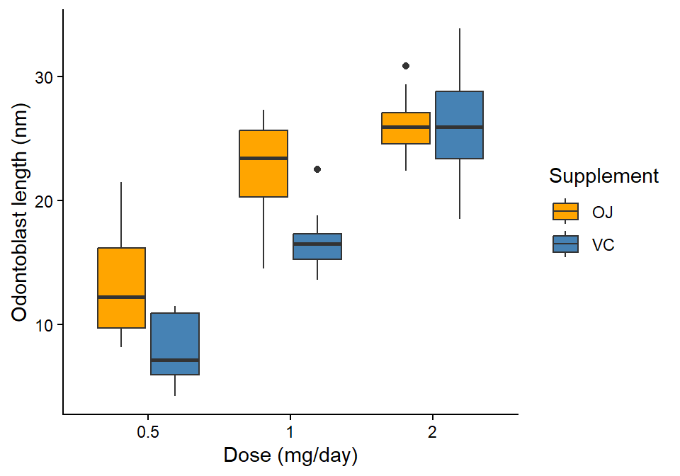

Figure 3: Odontoblast length by dosage and supplement type in guinea pigs.

Method 2: Specify group=

```{r}
#| code-fold: true
#| code-summary: "Method 2: Specify `group=`"
#| label: fig-lenByDose_gg2
#| fig-cap: "Odontoblast length by dosage and supplement type in guinea pigs."
#| fig-width: 5
#| fig-height: 3.5

ggplot(ToothGrowth, aes(dose, len, fill=supp, group=paste(dose, supp))) + 
  geom_boxplot() +
  scale_fill_manual("Supplement", values=c("orange", "steelblue")) +
  labs(x="Dose (mg/day)", 
       y="Odontoblast length (nm)")
```

Figure 4: Odontoblast length by dosage and supplement type in guinea pigs.

Scatter plots

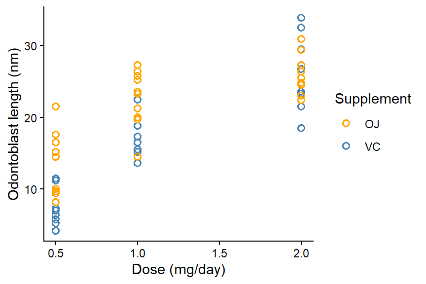
Using the same ToothGrowth dataset, produce a scatter plot of odontoblast length as a function of dose, where supp is the point colour.

Since supp is a factor, the levels can be coded into colours automatically in plot().

Using base R

plot(len ~ dose, data=ToothGrowth, col=supp,
     xlab="Dose (mg/day)",
     ylab="Odontoblast growth (AU)")
legend("topleft", 
       legend=levels(ToothGrowth$supp), 
       col=1:2, 
       pch=1, 
       bty="n")

Figure 5: Odontoblast length by dosage and supplement type in guinea pigs.

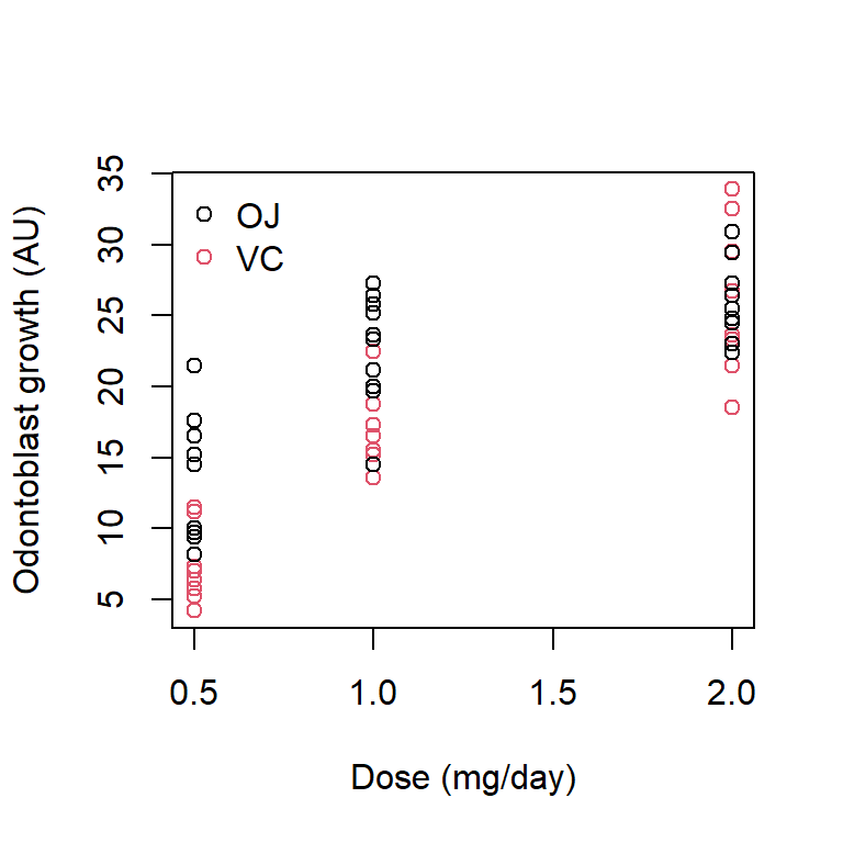
In my opinion, it is easier to use ggplot as your figures get more complex.

Using ggplot

ggplot(ToothGrowth, aes(dose, len, colour=supp)) + 
  geom_point(shape=1, size=2, stroke=0.8) +
  scale_colour_manual("Supplement", values=c("orange", "steelblue")) +
  labs(x="Dose (mg/day)", 
       y="Odontoblast length (nm)") +
  theme_classic()

Figure 6: Odontoblast length by dosage and supplement type in guinea pigs.