4 The t-distribution and confidence intervals
The goal of science is to understand the world (universe!). To do that, we want to know the values of population parameters (e.g., the mean size of barnacles on the back-beach, the variance in fail-rate of a machine component, the maximum satellite signal strength per satellite transect, the mean size of a fisher’s catch, …). However, we usually cannot measure entire populations due to logistical/time/money constraints. Instead, we take a (random) sample, and infer from that sample to our population of interest based on our statistical models of the world. This is statistical inference.
Unfortunately, we can never know how well our sample reflects the population.
For example, our random sample of barnacles might contain (by chance alone) mostly big ones, or barnacles that varied considerably (or negligibly) in size. The t-distribution is similar to the normal distribution, but it accounts for this added uncertainty. This enables us to estimate the probability that a given sample came from a population with any given mean (with caveats). The t-distribution also enables us to put confidence intervals around the mean of our sample, and gives us some idea of the values of the mean that are likely.
The t-distribution models the probability of making a given observation from a population whose parameters are estimated from your sample. The t statistic is calculated in the same way as the z score for samples, but the expected scores follow the t-distribution (instead of the normal distribution) which accounts for sampling uncertainty. For small sample sizes, we are less confident about the population parameter estimates, and the t-distribution consequently becomes shorter than the normal distribution and with fatter tails (Figure 4.1). The shape of the t-distribution depends on the degrees of freedom (\(df = \nu = N-1\)). There is more guidance on the t-distribution, and links to other sources on Brightspace.
Code (bonus)
t_Norm.df <- tibble(
  x = seq(-6, 6, length.out = 100),
  Norm = dnorm(x),
  t01 = dt(x, 1),
  t03 = dt(x, 3),
  t30 = dt(x, 30)
) |>
  pivot_longer(2:5, names_to = "distr", values_to = "Density") |>
  mutate(Distribution = factor(distr,
    levels = c("t01", "t03", "t30", "Norm"),
    labels = c("t(df=1)", "t(df=3)", "t(df=30)", "Normal(0,1)")
  ))

ggplot(t_Norm.df, aes(x, Density, colour = Distribution, linetype = Distribution)) +
  geom_line(linewidth = 1) +
  scale_colour_manual(values = c(RColorBrewer::brewer.pal(5, "BuGn")[2:4], "black")) +
  scale_linetype_manual(values = c(1, 1, 1, 3)) +
  theme_classic() +
  theme(legend.position = c(0.85, 0.8))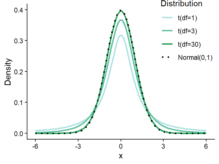
Q. 4.1
Would you feel as confident about basing an estimate of the heights of the lab population on a sample of 2 compared with a sample of 50?
Clearly not.
Q. 4.2
How does sample size affect the reliability of our population parameter estimates?
A larger sample leads to a more precise estimate (narrower confidence intervals) on average.
4.1 Single sample t-tests
The single sample t-test is analogous to the calculation of z scores. It enables us to determine how unlikely our sample mean is, given any hypothesized mean. However, before using any parametric tests such as t-tests, we need to assure ourselves that the model assumptions are reasonably met.
Imagine we are fisheries inspectors and have sampled the cod landed by a fishing boat. We know that the mean size of the landed cod should be greater than 36.6 cm. We need to assess how likely it is that our sampled cod come from a population where \(\mu \geq 36.6 cm\). We are testing the hypothesis that there is one ‘population’ of legally landed cod, and these cod are a part of that population. We use the t-distribution to assess the probability that our sample was drawn from a legally-landed cod population. If this probability is low then we might speculate that the cod are, in fact, drawn from a different population (i.e., that the boat is using illegal gear).
We do not know the mean \(\mu\) or standard deviation \(\sigma\) of the population and hence cannot use a normal distribution to model the likelihood of observing any particular value.
First, we should clearly state our hypotheses:
H0 (the null hypothesis): The population mean of the cod on this boat is greater than or equal to 36.6 cm (\(\mu \geq 36.6 cm\)).
H1 (the alternative hypothesis): The population mean of the cod on this boat is less than 36.6 cm (\(\mu < 36.6 cm\)).
We use a t-test to calculate the probability of drawing our sample from a population where the mean is 36.6 cm or greater.
Q. 4.3
Given the hypothesis, is this one or two tailed test?
One tailed.
We collect a sample of 20 fish (found in the worksheet ‘Cod lengths’). The sample size is \(<\) 30 so we can’t assume that the means will be normally distributed under the CLT. We can check the normality assumption by plotting the data using a ‘normality’ plot or ‘QQ-plot’ (Figure 4.2).
cod_df <- read_excel("data/H2SMS_practicalData.xlsx", sheet = "Cod lengths")
str(cod_df)
tibble [20 × 1] (S3: tbl_df/tbl/data.frame)
$ CodLength_cm: num [1:20] 34.1 35.6 36.1 34.6 38.3 35 36.8 38 34.4 35.5 ...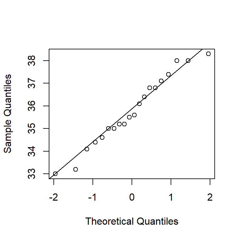
Q. 4.4
Do you think the normality assumption is reasonable?
Yes, the qqplot shows that the data are approximately normally distributed.
Q. 4.5
What parameter are we actually trying to understand? How does the distribution of the sample statistic change with sample size (think CLT)?
We are interested in the population mean \(\mu\), which we approximate using the sample mean \(\bar{y}\) which is our sample statistic. The distribution of possible sample means is centred on the population mean (assuming random samples), becomes narrower as sample size increases, and tends to be approximately normal when a) the data are approximately normal, or b) sample size is large enough (about 30 or more).
We wish to assess how likely our sample is to have been drawn from a population where \(\mu\) is at least 36.6 cm. If our sample mean \(\bar{y}\) is less than the ‘legal’ mean and it is ‘unlikely’ to have been drawn from a legal population, we might wonder if the mean of the landed cod on this boat is <36.6 cm and recommend legal action.
Q. 4.6
Q. 4.7
Q. 4.8
pt().
Code (bonus)
t.test(cod_df$CodLength_cm, mu = 36.6, alternative = "less")
    One Sample t-test

data:  cod_df$CodLength_cm
t = -2.3515, df = 19, p-value = 0.01482
alternative hypothesis: true mean is less than 36.6
95 percent confidence interval:
     -Inf 36.38429
sample estimates:
mean of x
   35.785
Hopefully your manually calculated t-statistic and the one generated by R match. The p-value given by R is exact: there is a probability of 0.014819 that a sample of 20 cod with mean of 35.785 cm would be drawn from a legally landed cod population where the true mean was 36.6 cm or more (assuming model assumptions are met).
Q. 4.10
What is your next step as the regulatory agent?
There is about a 1.5% chance of collecting a sample (n=20) with a mean this small if the population mean is 36.6 or more. You may thus conclude illegal practices, or a follow-up sample with a larger sample size.
Evaluating evidence is a central part of statistical analysis. In this example, your conclusion about the population mean \(\mu\) based on your sample determines whether legal action is taken. When a binary decision is necessary, it is best to set the decision threshold before collecting data. This is called the \(\alpha\) value. It is often set to 0.05, but this is a subjective choice. If \(P < \alpha\), the null hypothesis is rejected; the sample is considered too unlikely if \(\mu \geq 36.6cm\). In this scenario, we have two clear competing hypotheses, so we are in the realm of ‘Neyman-Pearson’s’ decision theory (not Fisher’s hypothesis significance testing approach).
Q. 4.11
Given the P value, do you reject the null hypothesis?
Yes, if \(\alpha = 0.05\).
Q. 4.12
If you had set \(\alpha\) at 0.01 would you reject the null hypothesis?
No.
Q. 4.13
If you set \(\alpha\) at 0.01 rather than 0.05, what type of error are you reducing and what type of error are you increasing? Which wrong conclusion becomes more likely and which becomes less likely?
Decreasing \(\alpha\) lowers the Type I error rate but raises the Type II error rate. You are less likely to falsely reject H0 but more likely to falsely ‘accept’ it.
Now let’s use simulation to explore variability among samples. We will repeatedly sample from \(y \sim Norm(100, 10)\).
Q. 4.14
What is the standard deviation in this model?
\(\sigma = 10\)
Q. 4.15
What does the symbol ‘~’ mean?
“Is modelled as”, “is distributed as”, or “is predicted by”
We will repeat our sampling num_samples times. Each sample will be sample_size values drawn from a normally distributed population with mean mu and standard deviation sigma. For each sample, we will calculate the sample mean \(\bar{y}\) and sample standard deviation \(s\). Note that in this case, we know the population parameters.
Copy the following code:
# set simulation details and population parameters
num_samples <- 5
sample_size <- 3
mu <- 100
sigma <- 10

# initialize plot
set.seed(1)
xlims <- c(mu-4.5*sigma, mu+3*sigma)
plot(NA, NA, xlim=xlims, ylim=c(0,num_samples),
     xlab="Observations", ylab="Sample number")
abline(v=mu, lty=3)
points(mu, 0, pch=4, col="steelblue")
segments(mu-sigma, 0, mu+sigma, 0, col="steelblue")
text(x=xlims[1], y=0, adj=c(0,0.5), col="steelblue",
     labels=paste0("mu: ", mu, ", sigma: ", sigma))

# repeatedly sample
for (i in 1:num_samples) {
  sample_i <- rnorm(n = sample_size, mean = mu, sd = sigma)
  sample_mean <- signif(mean(sample_i), 3)
  sample_sd <- signif(sd(sample_i), 3)
  # add to plot
  points(sample_i, rep(i, sample_size))
  points(sample_mean, i, pch=4)
  segments(sample_mean-sample_sd, i, sample_mean+sample_sd, i)
  text(x=xlims[1], y=i, adj=c(0,0.5),
       paste0("ybar: ", sample_mean, ", s: ", sample_sd))
}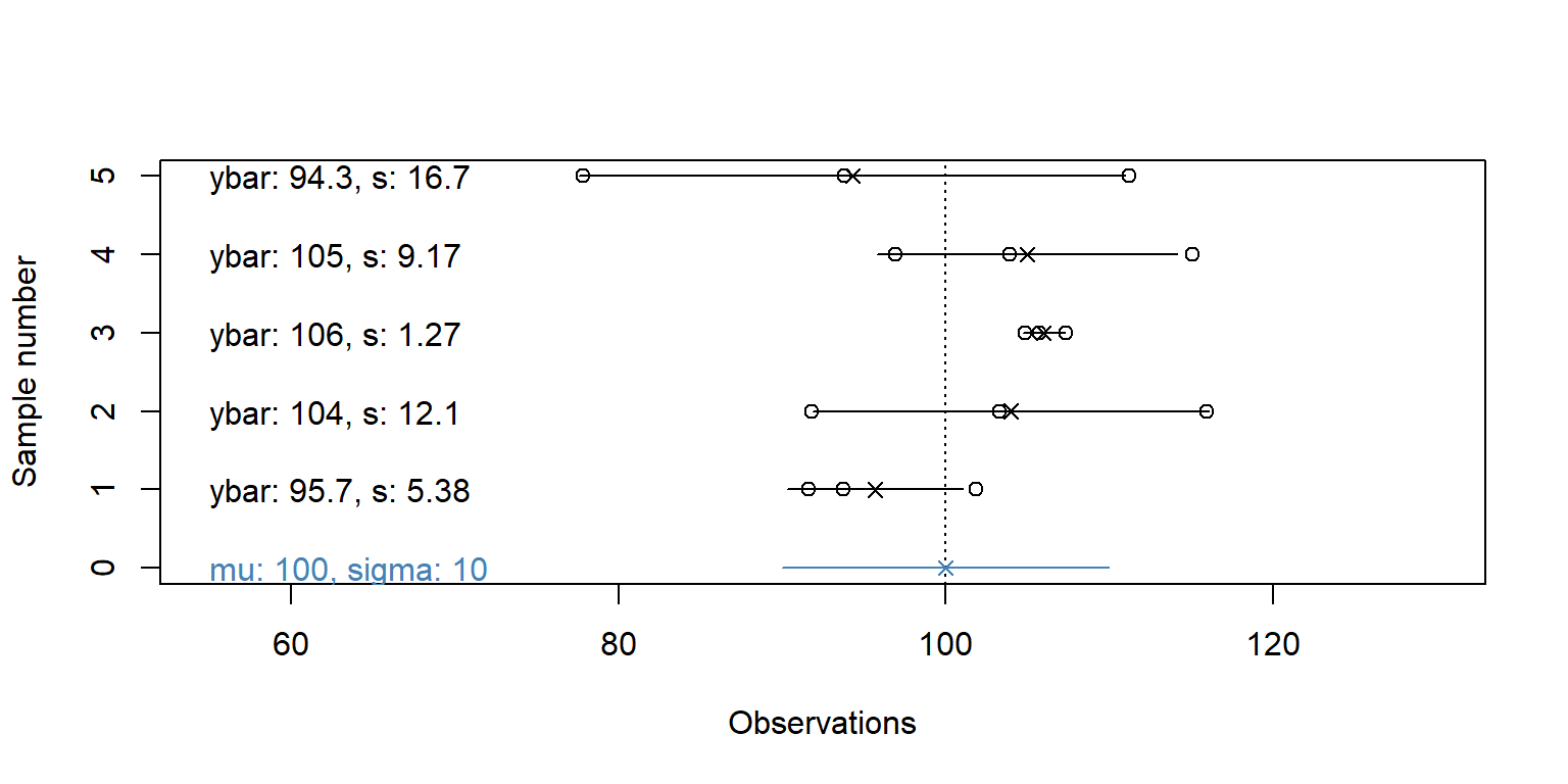
Note: these are random samples, so the values will be different each time you run the code. However, R uses pseudo-random number generation. Use set.seed() for fully reproducible code.
Q. 4.16
Is there a discrepancy between the population parameters and the sample statistics? Does the discrepency seem greater for the mean or the standard deviation?
Yes, there is a discrepancy. The relative variability in the sample standard deviation seems larger (often more than an order of magnitude between the smallest and largest estimates).
The discrepancy (\(\mu\) vs. \(\bar{y}\), \(\sigma\) vs. \(s\)) is called sampling error. In most situations, we do not know \(\mu\) and \(\sigma\), but must estimate them from our sample.
If the sample is very large (and representative) then the estimate of the population parameters is likely very good. However, as the sample size is reduced, the reliability of the estimate decreases. Try adjusting sample_size in the code above and see how it affects the results.
The t-distribution is the distribution of values you get when you subtract sample means from the population mean and standardize by the sample standard error (i.e., \(\frac{\bar{y} - \mu}{SE_{\bar{y}}}\)).
Q. 4.17
How does this distribution relate to the T-statistic calculated above? The P-value?
The T-statistic is the value from this distribution for a particular sample. The t-distribution gives the distribution of T-statistics we would expect for a given sample size if the null hypothesis were true. The P-value gives the area of this distribution that is more extreme than the specific T-statistic of interest.
We can extend the simulated sampling above to calculate a T-statistic for each sample in addition to \(\bar{y}\) and \(s\). We will set num_samples very large to better represent the distribution of sample T-statistics. The red histogram in Figure 4.4 shows the distribution of these sample T-statistics. The solid curve is the theoretical t-distribution (df=sample_size - 1) and the dotted line is a standard normal distribution.
Q. 4.18
Explore different values for sample_size below to see how the shapes change.
The distribution looks increasingly normal as sample_size increases. At small sample sizes, the peak is shorter and the tails are fatter because larger T-statistics are more likely.
Copy the following code:
mu <- 10 # population mean
sigma <- 10 # population sd
num_samples <- 1e5 # number of samples
sample_size <- 3 # size of each sample
T_sample <- numeric(num_samples) # sample t statistics

# for each repeat: draw a sample, calculate SE and T, and store T in T_sample
for(i in 1:num_samples) {
  sample_i <- rnorm(sample_size, mu, sigma)
  sample_SEM <- sd(sample_i) / sqrt(sample_size)
  T_sample[i] <- (mean(sample_i) - mu) / (sample_SEM)
}

curve(dnorm(x, 0, 1), from = -6, to = 6, lty = 2,
      xlab = "Simulated T-statistics", ylab = "Density",
      main = paste("T-statistics of",
                   format(num_samples, big.mark=",", scientific=F),
                   "samples, each with N =", sample_size))
hist(T_sample, freq = F, add = T, col = rgb(1, 0, 0, 0.25),
     breaks = seq(floor(min(T_sample)), ceiling(max(T_sample)), by=0.2))
curve(dnorm(x, 0, 1), from = -6, to = 6, add = T, lty = 2)
curve(dt(x, sample_size - 1), from = -6, to = 6, add = T)
legend("topright", lty = c(2, 1, 1), col = c(1, 1, 2), bty = "n",
       c("Normal(0,1)", paste0("t(df=", sample_size-1, ")"), "t-stat (sim)"))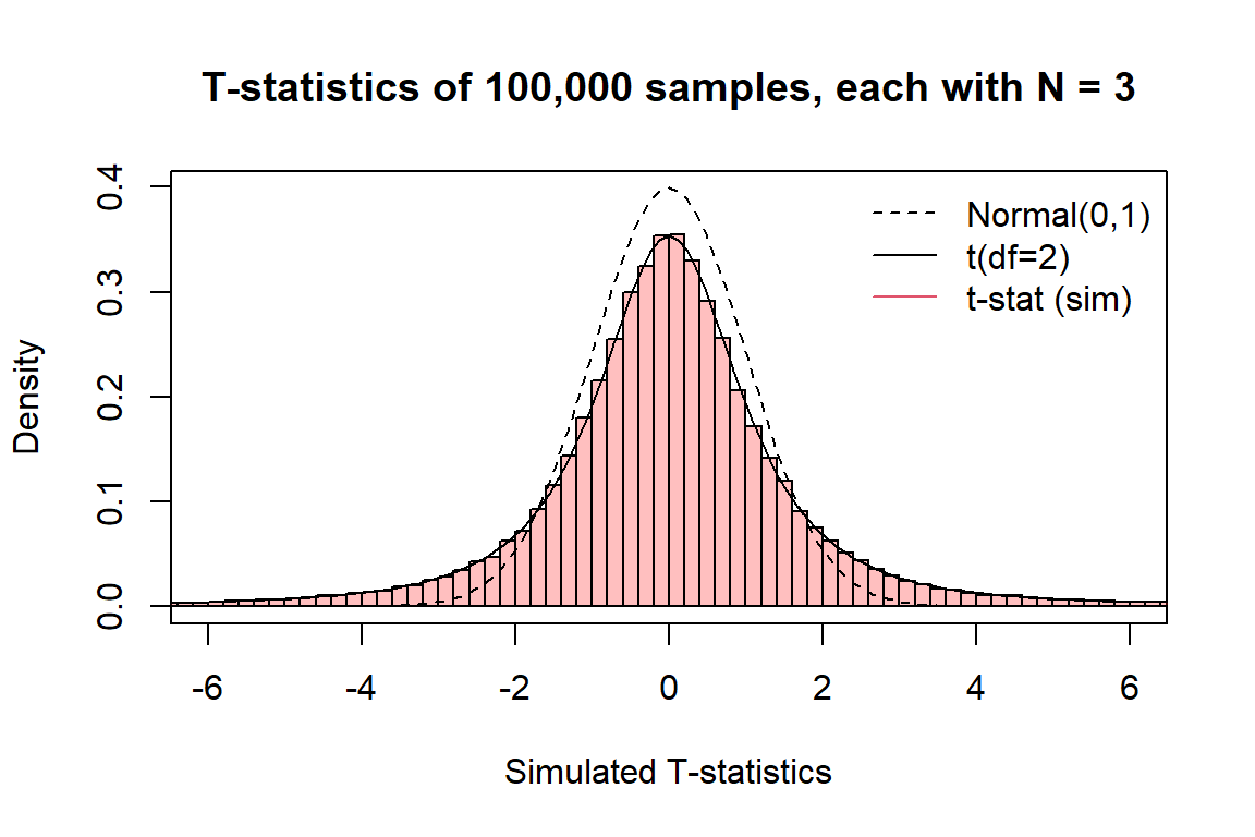
Notice how the histogram and the solid lines are nearly identical? These simulations illustrate that the t-distribution is the distribution of t-statistics for a given sample size.
When we perform a t-test, we compare the T-statistic from our sample to this distribution: the distribution of T-statistics we would expect under the hypothesized \(\mu\). The P-value gives the probability of our T-statistic (or one more extreme) under the hypothesized \(\mu\). If it is very small, it is very unlikely that our sample would occur with that \(\mu\), and we might conclude the value of \(\mu\) is something different.
4.2 Confidence Intervals
Say you are interested in knowing the mean of a population (e.g. barnacle mass on the back beach). You cannot afford to determine the mass of each barnacle, so you take a random sample. You don’t know how ‘good’ (i.e. representative) your sample is. It might have included lots of small barnacles, or big ones, or a wide- or narrow-range of sizes. You can never know (unless you sample everything). When you calculate the mean of this sample you don’t know how close it is to the population mean, but you do know the probability associated with that estimate. Confidence intervals capture this uncertainty, and you use the t-distribution to determine them.
We’ll invent a population of barnacle diameters, called barnacle_diam. We’ll create a histogram of that population and superimpose values on that. Again, these are random numbers so your values will be slightly different from mine.
# barnacle population meta-details
pop_size <- 100000  # number of barnacles in the population
barnacle_mu <- 200
barnacle_sigma <- 25

# the full population:
barnacle_diam <- rnorm(pop_size, mean = barnacle_mu, sd = barnacle_sigma)
mu <- mean(barnacle_diam)
sigma <- sd(barnacle_diam)

# histogram of the population with middle 95% shown
hist(barnacle_diam, main = NULL)
Q95 <- quantile(barnacle_diam, c(0.025, 0.975))
abline(v = Q95, col = "green", lwd = 3)
text(x=Q95[2], y=pop_size/7,
     labels=paste0("mu: ", round(mu, 1), "\nsigma:", round(sigma, 1)))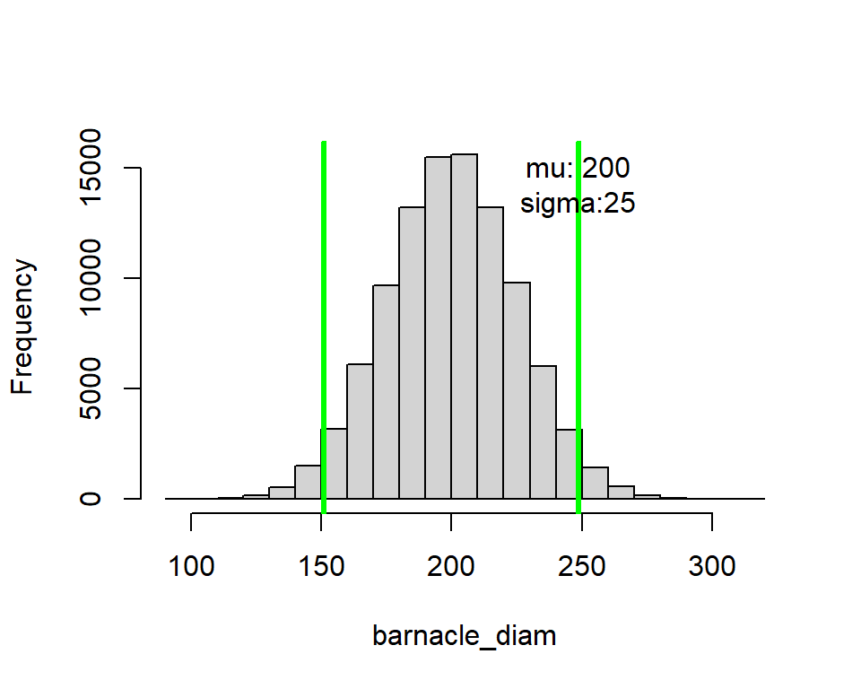
Now we can take samples from that population. This is reality: you take samples from populations where you don’t know the population mean and standard deviation. Let’s take 4 samples, each with size sample_size.
[1] 252.2560 209.5652 194.1364 180.0893 199.9900
[1] 181.4844 212.2622 212.0780 205.8330 209.9440
[1] 214.3341 150.0059 206.0774 194.1674 191.1762
[1] 168.1111 194.2603 180.3917 178.7273 193.4117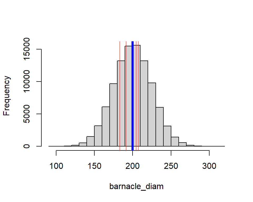
Our sample means inevitably differ from the true population mean (\(\mu\)), even if only a bit. Likewise, the sample standard deviations will differ from the true population standard deviation (\(\sigma\)).
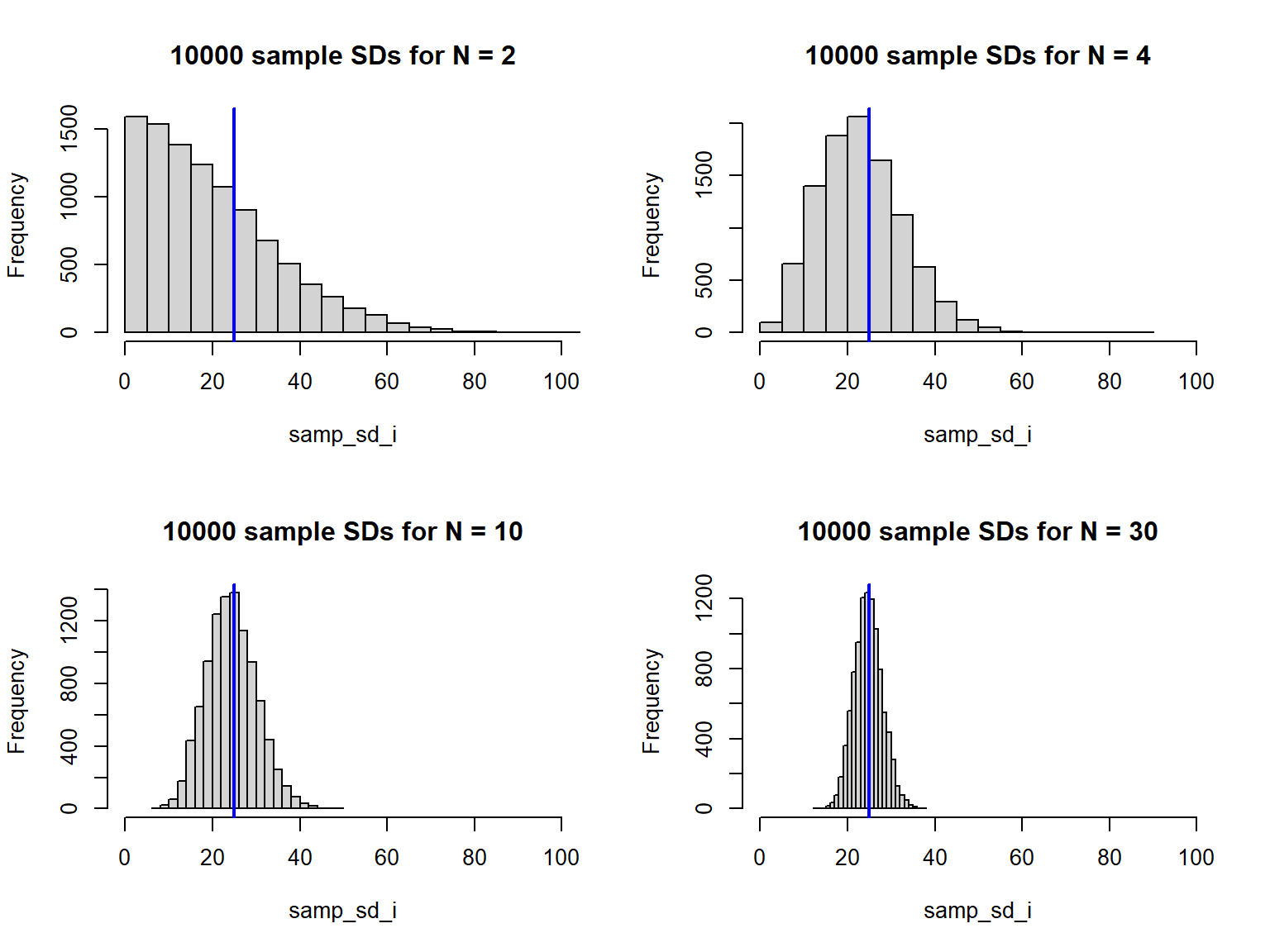
If we repeat this sampling enough times, we can generate a distribution of sample standard deviations (Figure 4.7). This distribution is not normal, but is instead related to the chi-square distribution (don’t worry too much about this). The point is that if your sample size is small, your estimate of the standard deviation is often very poor.
Code (bonus)
par(mfrow=c(2,2))
# sim_df will hold the sample sizes N, and the median and mean sample sd's
num_samples <- 1e4
sim_df <- data.frame(N=c(2, 4, 10, 30),
                     sd_median=NA, sd_mean=NA,
                     sd_q025=NA, sd_q25=NA, sd_q75=NA, sd_q975=NA,
                     mn_median=NA, mn_mean=NA,
                     mn_q025=NA, mn_q25=NA, mn_q75=NA, mn_q975=NA)

# for each sample size N, draw a sample and store its mean and sd
# repeat this num_samples times
# plot a histogram of the sample sd's, then store the mean and median
for (i in 1:nrow(sim_df)) {
  samp_sd_i <- numeric(num_samples)
  samp_mn_i <- numeric(num_samples)
  for (j in 1:num_samples) {
    sample_ij <- sample(barnacle_diam, size = sim_df$N[i])
    samp_sd_i[j] <- sd(sample_ij)
    samp_mn_i[j] <- mean(sample_ij)
  }
  hist(samp_sd_i, main = paste(num_samples, "sample SDs for N =", sim_df$N[i]),
       breaks = 20, xlim = c(0, 100))
  abline(v = sigma, col = "blue", lwd = 2)
  sim_df[i, 2:13] <- c(median(samp_sd_i), mean(samp_sd_i),
                       quantile(samp_sd_i, probs = c(0.025, 0.25, 0.75, 0.975)),
                       median(samp_mn_i), mean(samp_mn_i),
                       quantile(samp_mn_i, probs = c(0.025, 0.25, 0.75, 0.975)))
}
Code (bonus)
par(mfrow=c(1,2))
plot(sim_df$N, sim_df$sd_median, col = "dodgerblue",
  xlim = c(0, 30), ylim = range(c(sim_df[,2:7], sigma)),
  type = "b", xlab = "Sample size", ylab = "Standard deviation"
)
segments(sim_df$N, sim_df$sd_q25, sim_df$N, sim_df$sd_q75, lwd=2)
segments(sim_df$N, sim_df$sd_q025, sim_df$N, sim_df$sd_q975)
lines(sim_df$N, sim_df$sd_mean, type = "b")
abline(h = sigma, lty = 2)
legend("topright", c("Mean sample SD", "Median sample SD", "True SD"),
  col = c("black", "dodgerblue", "black"),
  lty = c(1, 1, 2), pch = c(1, 1, NA), bty = "n"
)
plot(sim_df$N, sim_df$mn_median, col = "dodgerblue",
  xlim = c(0, 30), ylim = range(c(sim_df[,8:13], mu)),
  type = "b", xlab = "Sample size", ylab = "Mean"
)
segments(sim_df$N, sim_df$mn_q25, sim_df$N, sim_df$mn_q75, lwd=2)
segments(sim_df$N, sim_df$mn_q025, sim_df$N, sim_df$mn_q975)
lines(sim_df$N, sim_df$mn_mean, type = "b")
abline(h = mu, lty = 2)
legend("topright", c("Mean sample mean", "Median sample mean", "True mean"),
  col = c("black", "dodgerblue", "black"),
  lty = c(1, 1, 2), pch = c(1, 1, NA), bty = "n"
)
Q. 4.19
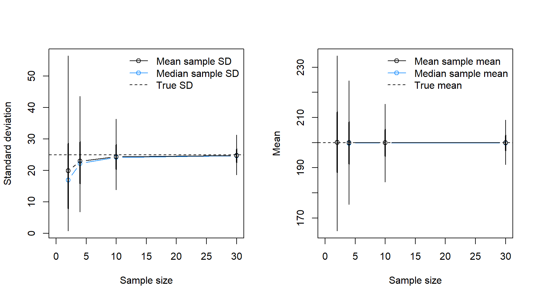
Does the difference between the mean (black) and median (blue) in Figure 4.8 match your expectations based on the shape of the distributions in Figure 4.7?
Yes. The distribution is skewed right, so the mean is larger than the median.
The t-distribution allows for the fact that the standard deviation of small samples is usually less than that of the population as seen in Figure 4.7 and Figure 4.8.
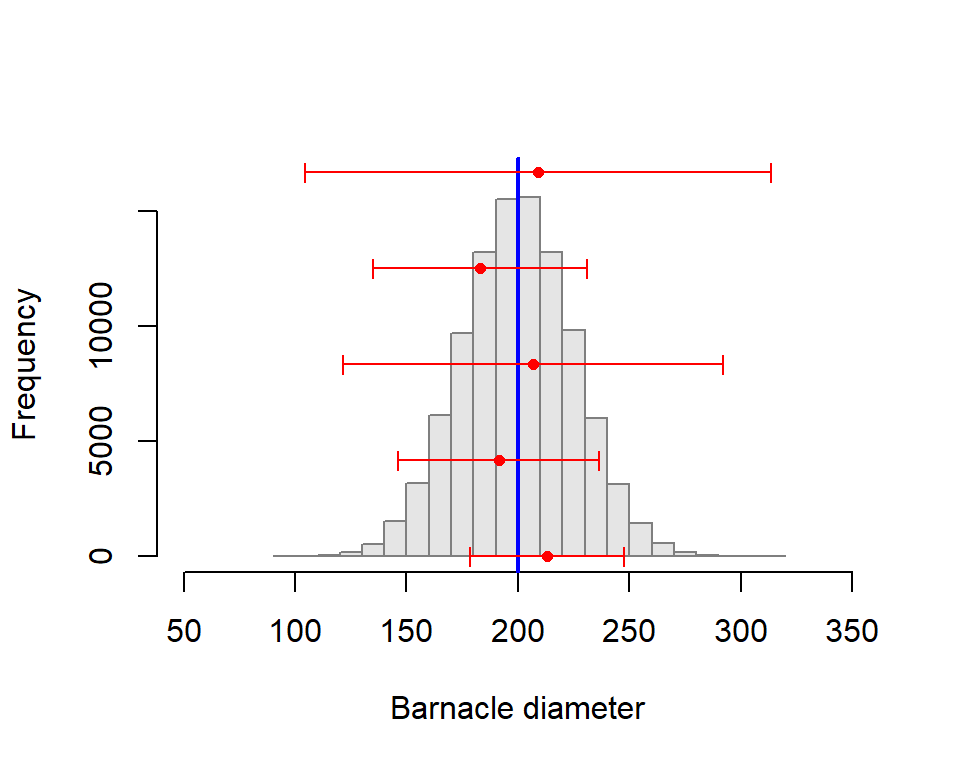
The take home message here is that when we sample from a population with unknown \(\mu\) and \(\sigma\), we won’t know how ‘accurate’ the sample is, but we do know how your random samples ‘behave’ - they are modelled using the t-distribution. From this knowledge, we can build a 95% confidence interval which is described as an interval which, if repeated for many samples, would include \(\mu\) within its boundaries in 95% of those samples. Read that again. You don’t have knowledge of the true value of the mean or sd (as you did for Z score calculations) and the t-distribution accounts for this uncertainty.
A 95% confidence interval is the interval that, when calculated on infinite repeated samples, contains the population mean for 95% of those samples (and thus misses the population mean in 5% of the samples).
We can modify Figure 4.6 by adding 95% confidence intervals for each sample from our barnacle population.
Copy the following code:
num_samples <- 5
sample_size <- 3

# plot population
hist(barnacle_diam,
     xlim = c(barnacle_mu-6*barnacle_sigma, barnacle_mu+6*barnacle_sigma),
     ylim = c(0, length(barnacle_diam)/6),
     main = NULL,
     col = "grey90", border = "grey50", xlab = "Barnacle diameter")
abline(v = mu, col = "blue", lwd = 2)
y_pos <- seq(0, length(barnacle_diam)/6, length.out=num_samples)

# draw samples, calculate mean and 95% CIs, and plot them
for (i in 1:num_samples) {
  sample_i <- sample(barnacle_diam, size = sample_size)
  points(x = mean(sample_i), y = y_pos[i], col = "red", pch = 16, cex = 0.75)
  sample_ci <- c(
    mean(sample_i) + qt(0.025, (sample_size - 1)) * (sd(sample_i) / sqrt(sample_size)),
    mean(sample_i) + qt(0.975, (sample_size - 1)) * (sd(sample_i) / sqrt(sample_size))
  )
  arrows(sample_ci[1], y_pos[i], sample_ci[2], y_pos[i],
         col = "red", code = 3, angle = 90, length=0.05)
}
Q. 4.20
Q. 4.21
Try different values for sample_size. How does this influence the width of your CIs?
Larger sample sizes produce narrower CIs on average.
Q. 4.22
What proportion of your 95% CIs would you expect to include the true value of the mean? Does that change for different values of sample_size?
95% of 95% CIs will capture the true value (on average) regardless of the sample size. This is how they are defined. Larger sample sizes decrease the width of the CIs but still result in 5% of samples having 95% CIs that miss the true value.
Q. 4.23
Find the relevant bit of the code and determine 99% CIs, then 79% CIs. Note that you may need to adjust the x-axis limits which are set to 6 \(\sigma\) on either side of \(\mu\) in hist()).
The first argument of qt() needs to be changed to 0.005 and 0.995 for 99% CIs and to 0.105 and 0.895 for 79% CIs.
Determine the percent that needs to be excluded, then divide that into upper and lower areas.
In the above code, we calculated CIs manually using qt(). We can instead simply use t.test() and specify whatever confidence level we like:
    One Sample t-test

data:  barnacle_sample
t = 35.493, df = 9, p-value = 5.533e-11
alternative hypothesis: true mean is not equal to 0
89 percent confidence interval:
 196.7245 217.4111
sample estimates:
mean of x
 207.0678
# Or just the confidence intervals:
examp_ttest$conf.int[1] 196.7245 217.4111
attr(,"conf.level")
[1] 0.89Let’s explore the influence of sample size on the width of the confidence interval a little more.
For sample sizes of 2, 5, and 10, we will collect a sample and calculate the 95% CIs with t.test(). As above, we will repeat our sampling a few times to assess the variability among samples of the same size.
Code (bonus)
num_samples <- 10
sample_sizes <- c(2, 5, 10)

CI_df <- expand_grid(N=sample_sizes,
                     sample_id=1:num_samples) |>
  rowwise() |>
  mutate(obs=list(sample(barnacle_diam, N)),
         mn=mean(obs),
         ci_lo=t.test(obs)$conf.int[1],
         ci_hi=t.test(obs)$conf.int[2]) |>
  ungroup() |>
  mutate(N=factor(N, levels=unique(N), labels=paste("N =", sample_sizes)))
ggplot(CI_df, aes(mn, sample_id, xmin=ci_lo, xmax=ci_hi, colour=N)) +
  geom_vline(xintercept=barnacle_mu, colour="cadetblue") +
  geom_point(size=1.5) +
  geom_errorbarh(height=0.15) +
  facet_wrap(~N, ncol=1, scales="free_y", strip.position="left") +
  labs(x="Sample mean and 95% confidence interval") +
  theme_bw() +
  theme(axis.text.y=element_blank(),
        axis.ticks.y=element_blank(),
        axis.title.y=element_blank(),
        legend.position="none",
        panel.grid.minor=element_blank())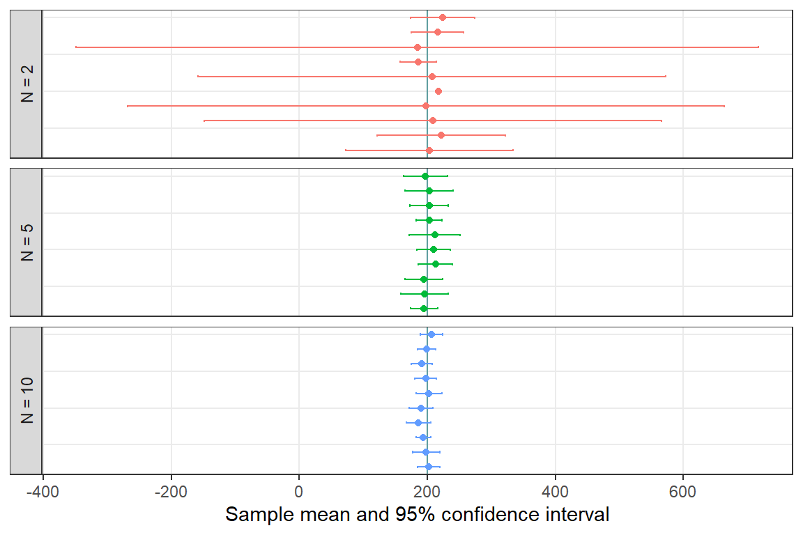
Q. 4.24
What do you notice about the average width of CIs in Figure 4.10 as sample size changes? What about the variability in width?
The average width decreases as sample size increases. The variability in width decreases as well.
Q. 4.25
What proportion of 95% CIs would you expect to include \(\mu\) for N=2? For N=100?
Always 95% no matter what the sample size is.
4.3 Comparing means (two-sample t tests)
The two-sample t-test is a widely used inferential statistical test. The two-sample t-test is a special case of analysis of variance (ANOVA) where there are only two groups. The results are identical and so we only mention its existence. It is good to be aware of the two-sample t-test because it is so commonly used, but you will be comparing means using ANOVA in ?sec-P5.
4.4 Non-parametric Tests
Parametric tests are so named because they estimate population parameters. Non-parametric tests are often used to compare samples where the data are non-continuous or fail the assumptions of parametric general linear models, typically converting data to ranks for analysis rather than using the actual values. Non-parametric test include ‘classics’ such as the ‘Mood’ and ‘Wilcoxon’ tests. However, we make you aware of the GLM family which will usually supply you with a much more elegant solution to model data that doesn’t fit the simple linear model. You should be aware of the existence of ‘non-parametric’ tests because they are prevalent in the literature. Remind yourself of the disadvantages of non-parametric tests.
4.5 Conclusions
The t-test is a ‘classic’ statistical test which doesn’t assume knowledge of population parameters. The strength of the t-test (its ability to quantify differences between samples) is proportional to the sample size. The larger the sample size, the better the estimate of the population parameters and the more precisely we are to be able to detect differences between the means.
The central limit theorem tells us that the means of non-normally distributed data will be normally distributed if the sample size is sufficiently large. If your sample size is \(>\) 30 it is likely that the means of that sample will be normally distributed regardless of the distribution of the original data.
Parametric tests including the t-test are quite ‘robust’ against deviations from normality, particularly as sample sizes increase. However, parametric test are less robust against heteroscedasticity, regardless of sample size. Always check this assumption and be prepared to transform the data if the assumption of homoscedasticity is not tenable (more of this in ?sec-P5).
The t-test is in the ‘general linear model’ family (which is a subset of the generalized linear modelling family). General linear models are usually used to model continuous data where residual error is approximately normal. If you have count data, you should start with a different member of the GLM family before trying transformations to acheive approximate normality. Non-parametric tests are frequently adopted when data do not conform to the assumptions of normality but they are invariably used for NHST with all the inherent problems with that approach.
A final reminder with regard to many statistical tests, including all in the GLM family: they make the assumption that data are independent. You must always ensure that your experimental design lends itself to making independent observations in relation to the question you are asking. This is the most critical and fundamental of the assumptions of parametric and non-parametric tests. Non-independence (e.g. measuring the same urchin over time) can be modelled using more complex ‘mixed’ models. Application of mixed modelling is beyond this course but you should be aware of the limitations of the techniques that you are learning and know where to go next.