2 Binomial and Poisson distributions
We often wish to determine the probability of events occurring given our current understanding of the processes involved. This requires a mathematical description of a theoretical relationship: a statistical model. Models are simplified representations of reality. As George Box said, ‘All models are wrong but some are useful’.
Two models, the binomial and Poisson distributions, often provide excellent approximations of real-world events. This means that they can be used to determine the likelihood of events or series of events given certain ‘reasonable’ assumptions. In terms of planning, e.g. in the insurance industry, this is extremely useful.
For example, the binomial or Poisson distributions can be used to answer:
- How likely is it that four hurricanes hit the US in one season based on historic data?
- How likely is it that a ‘50-year’ wave will hit in the next ten years?
- Is a river flooding more frequently now than it used to?
- What proportion of egg clutches in a fish population will be all males?
This practical gives you the opportunity to practice using these distributions.
2.1 The Binomial distribution
2.1.1 Bernoulli trials
A Bernoulli trial is a single event with a binary outcome (i.e., two categories that are mutually exclusive). Binary outcomes include:
- Alive vs. dead
- Reproductive vs. not reproductive
- Present vs. absent
Other variables can be re-coded into a binary outcome. For example:
- Flower colour (blue vs. not blue)
- Income (\(\geq\) £100,000 vs. \(<\) £100,000)
By definition, each Bernoulli trial is independent of all previous trials.
Q. 2.1
A fair coin has been heads in 99 consecutive flips. What is the probability of heads on the next flip?
0.5
This is different to asking whether (100 heads) or (99 heads + 1 tails) is more likely in a throw of 100 coins. Each single flip is an independent event.
2.1.2 The binomial distribution
The binomial distribution is a discrete probability distribution that applies to a series of Bernoulli trials.
For example, if a chicken laid 4 eggs and they were all female, you might wonder how likely this was by chance. Here, the outcome can be female or male, and the number of trials is 4: each egg is a ‘trial’ or ‘event’ with a binary outcome. You may question the assumption that the ratio of female:male was 50:50 and favour an alternative hypothesis that females are more likely. The binomial distribution allows you to quantify the probability of getting \(x\) females from \(n\) eggs for any given probability \(p=P(female)\). That is, we are not restricted to 50:50.
You need to know two things to use the binomial distribution. These are:
- The number of trials (\(n\), sometimes called \(k\))
- The probability of success (\(p\))
From p, we can calculate the probability of failure as \(q = (1-p)\), since the two probabilities must sum to 1.
The distribution of a binomially distributed variable \(y\) is specified as \(y \sim Binom(n,p)\). We denote \(P(x)\) as the probability of getting \(x\) successes where \(x\) is an integer from \(0\) to \(n\).
The mean of a binomial distribution is \(n*p\). This gives you the expected outcome. For example, if \(P(female)=0.5\) and \(n=4\) eggs the expected number of females is \(4*0.5=2\).
2.1.3 Binomial calculations
2.1.3.1 Sand tiger sharks
Sand tiger shark (Carcharias taurus) females have two uterine horns, each with as many as 50 embryos. However, they display ‘embryophagy’, where the largest embryo in each uterine horn eats all of the smaller embryos, so that females typically give birth to two pups.
Assume that the average sex ratio of sand tiger shark pups is 50:50. We are interested in the proportion of pups we expect to be female from one clutch (two pups).
Q. 2.2
What is the event?
Each pup – whether or not it is female.
Q. 2.3
What is \(p\)?
0.5
Q. 2.4
What is the number of trials?
2
Q. 2.5
How many possible outcomes are there for a clutch? What are they?
Three:
- two female
- one female, one male
- two male
Q. 2.6
Write down the model specification with parameters (i.e., \(y \sim Binom(...)\)).
\(y \sim Binomial(n=k=2, p=0.5)\)
Q. 2.7
Calculate the expected proportions of clutches that contain (a) two female, (b) two male, and (c) one of each. Use a probability tree if needed.
- 1/4
- 1/4
- 1/2
2.1.3.2 Great white sharks
Great white sharks (Carcharodon carcharias) typically give birth to 2-10 pups at a time. You’ve captured a female for tagging and found that she has 8 developing embryos.
We are interested in the proportion of pups we expect to be female from this shark’s clutch (8 pups).
Q. 2.8
What is the Bernoulli event?
Each offspring: Is it male or female?
Q. 2.9
What are the theoretical limits to your outcomes (i.e, max numbers of each)?
0 to 8
Q. 2.10
What are the possible outcomes? What is the number of possible outcomes?
0F 8M, 1F 7M, …, 8F 0M = 9 outcomes
Assume that the average sex ratio is even, such that the probability \(p\) of any offspring being female is 0.5 and being male \(q\) is 0.5. For the extreme cases where all offspring are one sex, we can use simple probability theory: the probability of getting \(n\) females in a brood of size \(n\) is equal to \(p^n\).
Q. 2.11
Write down the model for the number of female pups for this shark’s brood: \(y \sim Binom(n,p)\).
\(y \sim Binom(8, 0.5)\)
Q. 2.12
Calculate the probability of obtaining eight male offspring.
Could use the binomial formula, but the coefficient reduces to 1 since there is only one pathway to 8 males:
0.5^8[1] 0.00390625Q. 2.13
What is the mean number of females you would expect in great white shark broods of 8 pups?
With p=0.5, expectation is 4
It gets more complicated when you want to know the probability of getting, say, 1 male and 7 females from a brood of eight pups.
Q. 2.14
Given that \(p=q\), what shape would expect the distribution to be?
Symmetric
R can calculate probabilities for specific outcomes from a massive array of theoretical probability distributions, including the binomial distribution.
For ease, we can save the binomial distribution parameters as objects:
num_pups <- 8
p_female <- 0.5
To calculate the probability of 4 females:
# for a single probability: y~Binom(n=8, p=0.5) determine P(y_i=4)
dbinom(4, num_pups, p_female) # dbinom(4, 8, 0.5)
The function dbinom() gives the probability of a single outcome.
Often we want to know cumulative probabilities instead. This allows us to answer questions like “What is the probability of obtaining < 4 females in a brood of 8 pups?” Here, <4 equates to the cumulative probability P(0) + P(1) + P(2) + P(3).
In this case, we can use either pbinom(...) or sum(dbinom(...)) to give the cumulative probability.
[1] 0.00390625 0.03125000 0.10937500 0.21875000
[1] 0.3632813pbinom(3, num_pups, p_female)[1] 0.3632813Q. 2.15
Why do we parameterise pbinom() with 3 rather than 4?
pbinom(x, n, p) gives the cumulative probability up to and including x, and in this case we want to know less than 4 instead of less than or equal to 4.
Q. 2.16
Update the code to calculate \(P( \leq 4)\)?
pbinom(4, num_pups, p_female)[1] 0.6367187Q. 2.18
What is the probability of getting 3 females?
dbinom(3, num_pups, p_female)[1] 0.21875Q. 2.19
What is the probability of getting 8 females?
dbinom(8, num_pups, p_female)[1] 0.00390625Q. 2.20
What cumulative probabilities would you need to consider to answer the question “What is the probability of getting fewer than three females?”
From 0 to 2, which could be calculated with pbinom(2, num_pups, p_female)
Q. 2.21
Q. 2.22
What is the probability of getting < 6 females?
pbinom(5, num_pups, p_female)[1] 0.8554688Q. 2.23
What is the probability of getting \(\leq\) 6 females?
pbinom(6, num_pups, p_female)[1] 0.9648438Q. 2.24
What is the probability of getting > than 8 females?
0
Let’s visualize these distributions in order to better understand them.
# Run this, then explore values of p_female
# Note: 'success' and 'failure' is arbitrary. Just make sure you're calculating
# what you think. How would you calculate the probabilities for males instead?
num_female <- 0:8
p_female <- 0.5 # what are the limits of p_female?
prFemale_df <- data.frame(num_female=num_female,
                          prob=dbinom(num_female, max(num_female), p_female))
prFemale_df
num_female prob
1 0 0.00390625
2 1 0.03125000
3 2 0.10937500
4 3 0.21875000
5 4 0.27343750
6 5 0.21875000
7 6 0.10937500
8 7 0.03125000
9 8 0.00390625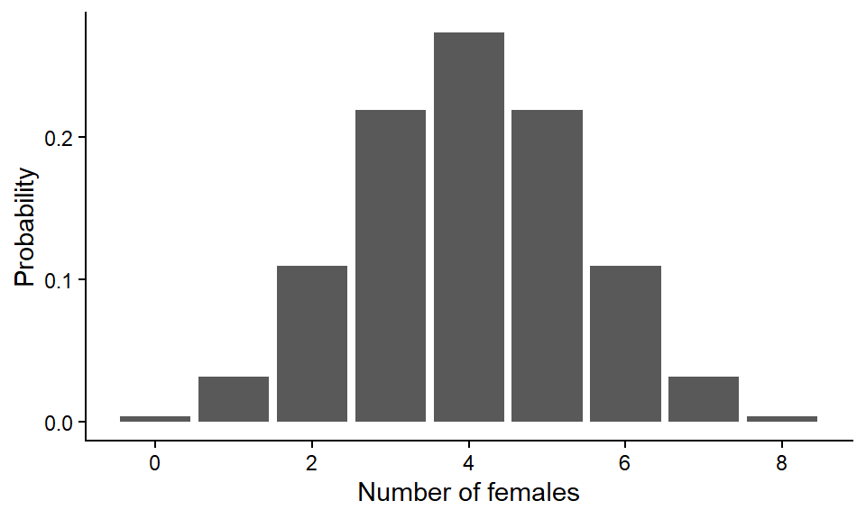
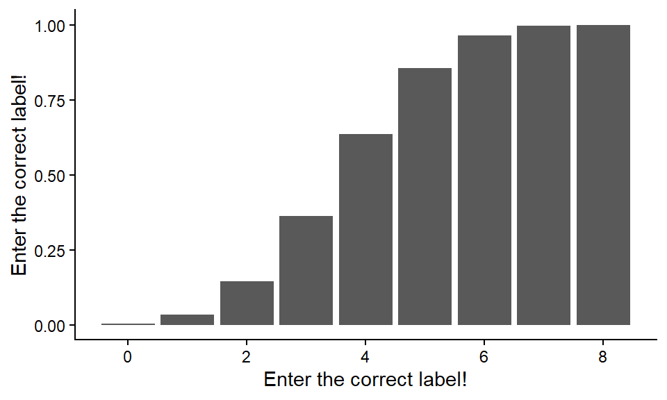
Try re-plotting so that the two panels appear side by side (hint: library(cowplot), then ?plot_grid).
Note \(P(y_i=x)\) is read as ‘the probability that y sub i equals x’. Sometimes this includes conditions: \(P(y_i=x|n,p)\), which is read as the probability that \(y_i\) equals \(x\) given \(n\) and \(p\). You may see \(P()\), \(Pr()\), \(p()\), or \(Prob()\), which all mean the same thing.
The interpretation of \(P(y_i=8\ |\ n=8,\ p=0.5) = 0.00391\) is that, in a brood of 8 pups where each pup has 50% probability of being female, the probability that all are 8 female is 0.00391.
In other words, if we have 500 broods, each with 8 pups, we expect \(500 * 0.00391 = 1.95 \approx 2\) broods to be all female. You wonderously manage to identify the sex of your shark’s pups, and find that all 8 are, in fact, female. Is there something strange about your shark or is it just one of the 2/500 by chance?
Q. 2.26
Why is a bar graph the appropriate plot here?
The outcome is a discrete variable: integers.
Q. 2.27
What do you notice about the shape of the distribution when \(p=q=0.5\)
It is symmetric.
Q. 2.28
Re-run the analysis with the probability of female as 0.8 and plot the results. How has the shape of the distribution changed?
The distribution is skewed left, with more probability mass toward larger numbers.
num_female <- 0:8
p_female <- 0.8
prFemale_df <- data.frame(num_female=num_female,
                          prob=dbinom(num_female, max(num_female), p_female))
prFemale_df$cumul_prob <- cumsum(prFemale_df$prob)
prFemale_df
num_female prob cumul_prob
1 0 0.00000256 0.00000256
2 1 0.00008192 0.00008448
3 2 0.00114688 0.00123136
4 3 0.00917504 0.01040640
5 4 0.04587520 0.05628160
6 5 0.14680064 0.20308224
7 6 0.29360128 0.49668352
8 7 0.33554432 0.83222784
9 8 0.16777216 1.00000000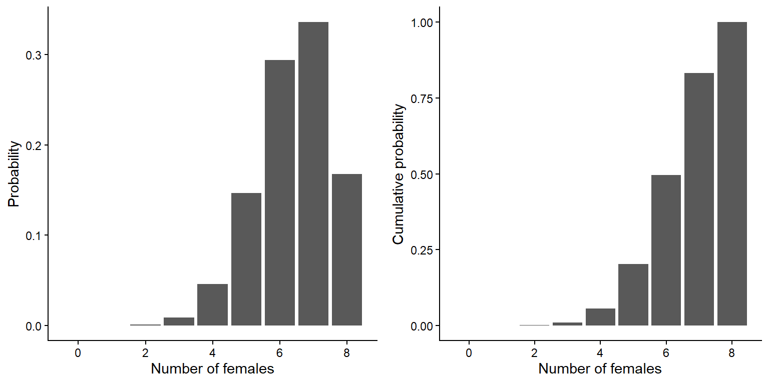
2.2 The Poisson distribution
The Poisson distribution is another probability distribution that describes discrete events that occur in space and/or time. The Poisson distribution is used to model (predict) the distribution of events that are rare, random, and independent. This can include events like earthquakes, storms, or the number of whales spotted on a cruise.
The Poisson distribution takes a single parameter: the mean. If a variable is Poisson distributed, its variance will equal its mean. This is a diagnostic feature of the distribution. The Poisson distribution is a discrete probability distribution, but its parameter, the mean, is continuous (similar to continuous \(p\) for the discrete binomial distribution).
Find the formula for the Poisson distribution in Chapter 5.
Here, \(\bar{y}\) is the mean, \(x\) is the outcome of interest, \(e\) is Euler’s number, and \(!\) is factorial. Note that here, we use \(\bar{y}\) as our stand-in for the population parameter \(\lambda = \mu = \sigma^2\) which defines the Poisson distribution.
Q. 2.29
Translate the Poisson formula into an R function by completing the following code.
calc_poisson_prob <- function(x, y_bar) {
  # Translate the formula here using x and y_bar
}
Hint 1
# In R, e^2 = exp(2)Hint 2
# In R, 3! = factorial(3)2.2.1 Poisson distributions by hand
When using the Poisson distribution, the first step is to calculate the mean number of observations per unit. This is the Poisson parameter, and is referred to as the rate or as lambda (\(\lambda\)). The unit could be spatial (e.g., per \(m^2\)) or temporal (e.g., per hour).
Last weekend, I randomly threw a 1\(m^2\) quadrat repeatedly on a sandy beach covered in worm casts Figure 2.3. In each quadrat, I counted the number of casts.
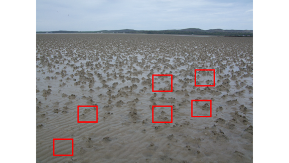
My observations can be found in the “WormCasts” sheet in “H2SMS_practicalData.xlsx”. Read in the data and calculate the mean number of worm casts per quadrat as well as the range of observations.
worm_df <- read_excel("data/H2SMS_practicalData.xlsx", sheet="WormCasts")
head(worm_df)
# A tibble: 6 × 2
quadrat casts
<dbl> <dbl>
1 1 0
2 2 0
3 3 1
4 4 1
5 5 0
6 6 1You should find a mean of 1.17, with values ranging between 0-6.
mean_casts <- mean(worm_df$casts)We wish to predict the proportion of quadrats that would contain 0, 1, 2, 3, 4, 5, and 6 worms, assuming that the worms are independently distributed across space (i.e., random: one worm’s location has no effect on another worm’s location, and there is no relevant environmental variation).
We will then compare our observations to the expectations from the theoretical Poisson distribution. To do this, we need to know the probability of observing each count, given the mean count per quadrat.
As the number of worms per quadrat is relatively small, the occurrences are rare enough to be reasonably described by a Poisson distribution if worms occur independently.
From the mean, we can calculate the expected frequency of observing different numbers of worms in any quadrat (assuming the model assumptions are met: What are the assumptions?). The number of worms per quadrat (\(y\)) is discrete; it can only take integers greater or equal to zero.
We are often interested in probabilities such as \(P(y_i \leq a)\). That is, the probability that an observation \(i\) of the random variable \(y\) is less than or equal to \(a\). For example, you may need to calculate \(P(y_i \leq 1)\), which is the probability that a random quadrat (\(y_i\)) contains 1 or fewer worm casts (\(a\), an integer value). To be fully complete, we might even write \(P(y_i \leq 1 | \bar{y})\), which acknowledges that we know the (sample) mean.
So, to calculate the probability of obtaining 1 or fewer worms per quadrat, you could start by writing \(P(y_i = 0) + P(y_i=1) = \dots\).
Q. 2.30
Use your calc_poisson_prob() function to calculate the expected frequency of 0, 1 & 2 worms per quadrat.
calc_poisson_prob(x=0:2, y_bar=mean_casts)[1] 0.3103669 0.3631293 0.2124307Q. 2.31
What calculation would you need to conduct to determine \(P(y_i \geq 1)\)? What is the theoretical upper limit of the Poisson distribution?
The upper limit is positive infinity, so to fully calculate the probability, use \(1 - P(y_i < 1)\)
R has built-in functions for calculating these, but it is important to know what you are asking them to calculate.
2.2.2 Poisson distributions using *pois() functions
You can determine the expected probabilities for each worm count per quadrat using the mean count of worms per quadrat.
Given this, we can find \(P(y_i \leq 5)\): the probability of a random quadrat containing five or fewer worms. With a mean of 1.17 worms per quadrat, \(P(y_i \leq 5) = 0.999\) (3 sf). This means that if your data are Poisson distributed with \(\lambda = 1.17\), it is highly unlikely to find more than five worms in a quadrat.
To do these calculation in R, we can use dpois() and ppois():
# ?dpois
# for questions like 'determine P(y_i=a | lambda)'
a <- 5
lambda <- 1.17
dpois(a, lambda) # probability of observing 'a' worms per quadrat: dpois()
[1] 0.005670528# ?ppois
# for questions like 'determine P(y_i >= a | lambda)
1-ppois(a-1, lambda) # probability of observing >= 'a' worms: ppois()[1] 0.006992103Q. 2.33
Why is a-1 used in the ppois() function above? When would you use a instead?
As with pbinom(), the specified value is included in the sum. So we would use a instead of a-1 if we were interested in \(P(y_i \leq a)\) instead of \(P(y_i < a)\).
For the converse (greater than, as in the example above), the same logic applies.
ppois(0:a, mean_casts) # what does 0:a mean? What's another way to make this vector? [1] 0.3103669 0.6734963 0.8859269 0.9687749 0.9930079 0.9986784[1] 0.310 0.673 0.886 0.969 0.993 0.999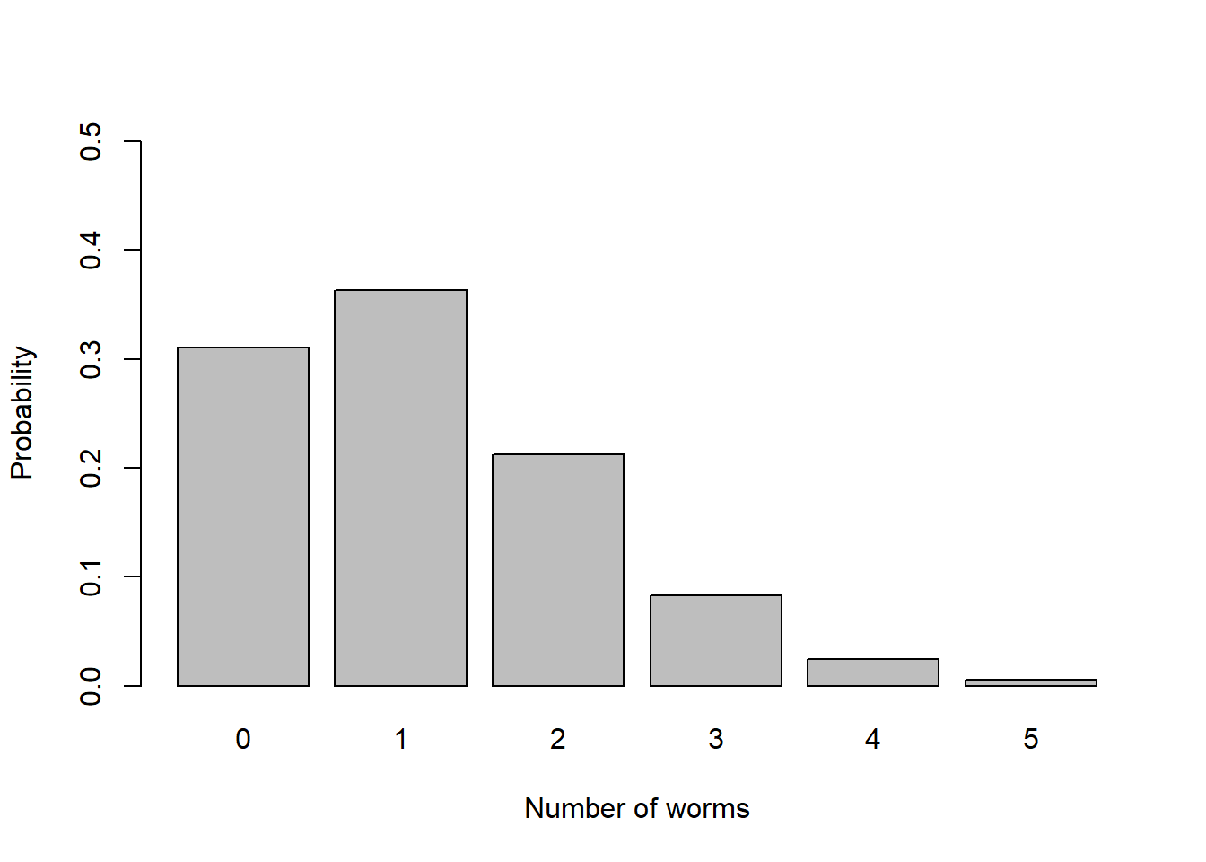
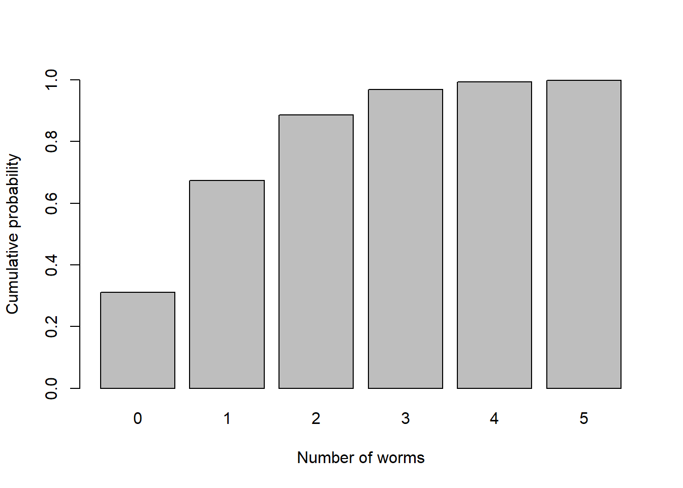
To compare my observations with these theoretical Poisson expectations, we need to tally the number of 0, 1, etc worms. The easiest way is with count().
# Make Table 2.1. Use packageName::function() instead of loading with library()
knitr::kable(worm_summary, digits=5) | casts | n | prob | cumul_prob |
|---|---|---|---|
| 0 | 33 | 0.31037 | 0.31037 |
| 1 | 37 | 0.36313 | 0.67350 |
| 2 | 16 | 0.21243 | 0.88593 |
| 3 | 9 | 0.08285 | 0.96877 |
| 4 | 4 | 0.02423 | 0.99301 |
| 5 | 1 | 0.00567 | 0.99868 |
If individual probability values (not cumulative probability) are multiplied by the total number of quadrats thrown (n=100), we generate the expected frequency distribution for comparison with the observed results above.
Q. 2.36
Write the appropriate code to add a column (called n_expected) to worm_summary that is the expected number of quadrats (given 100 quadrats total).
worm_summary$n_expected <- 100 * worm_summary$probThis is the number of quadrats that you would expect to contain 0, 1, …, 5 worms, given that the mean density of worms is 1.17 per m\(^2\). Note that the number of worms per quadrat is a discrete variable, but you can have non-integer ‘expectations’ (i.e. means).
Q. 2.37
Add another column that is the difference in the observed number of quadrats and n_expected.
worm_summary$diff <- worm_summary$n - worm_summary$n_expected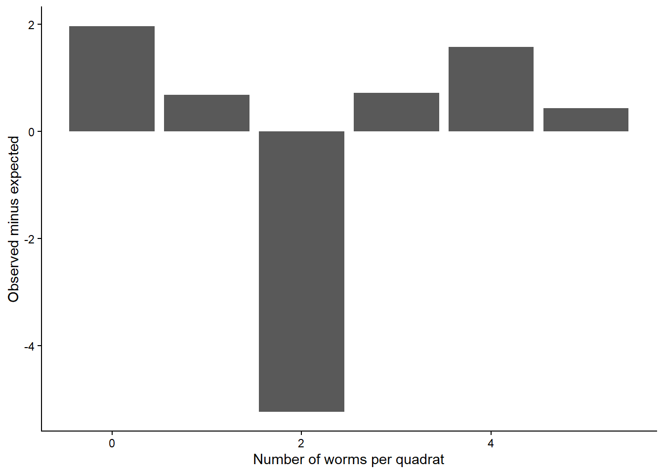
Q. 2.39
Calculate the observed variance. Do these observations tend to be overdispersed or underdispersed (= clumped)?
var(worm_df$casts)[1] 1.354646They tend to be overdispersed, with higher variance than expected under a Poisson distribution. That is, there are more low and high values than predicted and fewer intermediate values than expected.
Here is a figure showing the distributions side-by-side:
Code (bonus)
worm_summary |>
  select(casts, n, n_expected) |>
  pivot_longer(2:3) |>
  ggplot(aes(casts, value, fill=name)) +
  geom_bar(stat="identity", position="dodge", colour="grey30") +
  scale_fill_manual("Distribution",
                    values=c("cornsilk2", "cornsilk4"),
                    labels=c("Observed", "Expected")) +
  labs(x="Number of worms per quadrat",
       y="Number of quadrats") +
  theme(legend.position="inside",
        legend.position.inside=c(0.9, 0.9))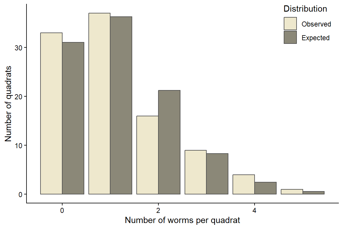
2.3 The Poisson approximation of the binomial model
When the number of trials \(n\) is large and the probability of success \(p\) is small, the Poisson distribution can be used as an approximation of the binomial distribution. Under these circumstances you can calculate the mean of a variable that has a binomial distribution (\(n*p\)) and use that to approximate \(y \sim Pois(\lambda = np)\). Using the Poisson distribution is computationally more efficient in these cases. There is no settled threshold, but as \(n\) increases and \(p\) decreases, the approximation gets better.
If we set the mean \(\lambda = np = 5\), we can visualize the distributions with different combinations of \(n\) and \(p\) (e.g., \(p=0.5, n=10\); \(p=0.05, n=100\), etc). We can use this to illustrate how the binomial distribution converges to the Poisson distribution as \(n\) gets larger.
Code (bonus)
# generate dataframe with probability for 0:16 'successes' from different
# distributions but where mean is 5.
# note that in y ~ Binom(10,0.5), probability of >10 successes is zero.
y_seq <- 0:13
binom_df <- tibble(y=rep(y_seq, times=4), # ?rep
                   n=rep(c(10, 20, 100, 500), each=length(y_seq)),
                   p=rep(c(0.5, 0.25, 0.05, 0.01), each=length(y_seq))) |>
    mutate(mean=n*p,
           prob=dbinom(y_seq, n, p),
           label=paste0("y ~ Binom(", n, ", ", p, ")"))
pois_df <- tibble(y=y_seq,
                  n=NA,
                  p=NA,
                  mean=5) |>
    mutate(prob=dpois(y_seq, mean),
           label=paste0("y ~ Pois(", mean, ")"))
distr_df <- bind_rows(binom_df, pois_df) |>
  mutate(label=factor(label, levels=unique(label)))
Code (bonus)
ggplot(distr_df, aes(y, prob, fill=label)) +  # ggplot(data, aes(xVar, yVar))
  geom_bar(stat="identity", position="dodge", colour="grey30") +  # ?geom_bar
  scale_fill_brewer("Distribution", palette="PuBu") + # from colorbrewer2.org
  labs(x="Number of successes with mean = 5", y="Probability") +
  scale_x_continuous(breaks=y_seq) +
  theme_classic() +
  theme(legend.position=c(0.85, 0.85))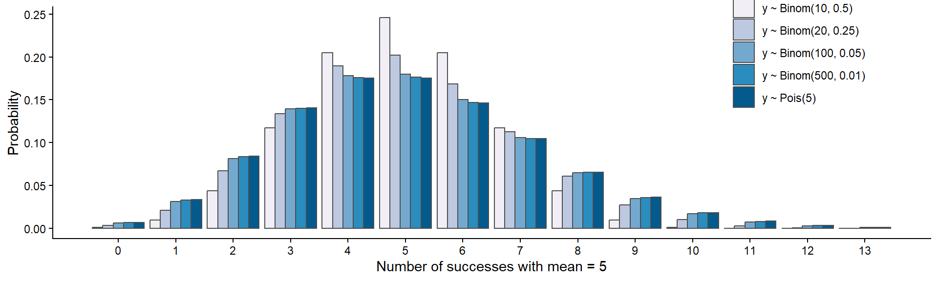
Q. 2.40
What is the modal value in each of these distributions?
5 in all cases.
Q. 2.41
Generate some random numbers from the distributions in Figure 2.5 and calculate their mean and variance.
[1] "Mean: 4.98, variance: 2.56"[1] "Mean: 5.01, variance: 3.67"[1] "Mean: 4.97, variance: 4.73"[1] "Mean: 4.96, variance: 4.37"[1] "Mean: 4.98, variance: 4.96"Here is \(y \sim Pois(\lambda=5)\):
[1] "Mean: 5, variance: 5.19"Q. 2.42
What do you notice about the mean and variance in the Poisson model?
They are very similar, but not identical since this is a sample.
Q. 2.43
What do you notice about the mean and variance in the binomial models as \(n\) increases and \(p\) decreases? When is it more similar to the Poisson? Is this what you expected?
They become increasingly similar. Yes, this is expected because this is what the text above says and we (briefly) discussed it in the lecture.
2.4 Conclusions
The binomial distribution is a discrete probability distribution that models situations where the outcome of an observation or experiment is binary (i.e., two possibilities) or is coded as such. The binomial model enables us to predict the probability of making our observation or series of independent observations for any given probability of a success (\(p\)) in a known number of trials. This enables us to quantify how likely our observation is to have occurred by chance. If the chance of our observation is very low, we can challenge the hypothesis with regard to the probability of success (\(p\)) and suggest a different value.
The Poisson distribution is another discrete probability distribution that is used to predict the probability of counts that are rare, independent and randomly distributed with mean = variance = \(\lambda\). The Poisson distribution can be used as an approximation of the binomial distribution where the number of trials (\(n\)) is large and the probability of success (\(p\)) is small. This approximation is useful as, unlike the Poisson distribution, the binomial calculation requires the handling of massive numbers (from large factorials).