Problem Set 2

Please render this file to .html and submit via Brightspace.

library(tidyverse); theme_set(theme_classic())
library(readxl)
set.seed(2026)

Binomial distribution

Scenario 1

Alex is interested in how likely their tulip bulbs are to flower in their garden. They buy three identical packages of five bulbs from Tesco and plant them in November. In April, they see that 12 have successfully produced flowers.

What is \(k=n\)?

k=n

k <- 15
k

[1] 15

What is their best estimate for the probability that a given tulip bulb will flower (\(\hat{p}\))?

p-hat

p_hat <- 12/k
p_hat

[1] 0.8

What is the standard error on this sample proportion?

Standard error

sqrt( (p_hat*(1-p_hat))/(k-1) )

[1] 0.1069045

Scenario 2

Mary is interested in the effect of winter storms on the detachment rates of the kelp Laminaria hyperborea. She is studying a small population near the beach at Wee Ganavan with \(n=22\) individuals forming the canopy. She reads that in similar locations, storms cause an average of 39.4% of canopy plants to dislodge over the winter.

Using these values, what is the mean expected number of dislodged plants in her population?

Mean expected dislodgement

p <- 0.394
k <- 22
p*k

[1] 8.668

Make a barplot showing the probability of each possible number dislodged individuals.

Bar plot (ggplot)

# Here I created a dataframe (tibble) 'on the fly' using a pipe |> instead
# of storing it as an object. I'm only using it for the plot, so don't really
# care to keep it around in my R environment
tibble(nDislodged=0:k,
       prob=dbinom(nDislodged, k, p)) |>
  ggplot(aes(nDislodged, prob)) + 
  geom_bar(stat="identity") +
  labs(x="Number of dislodged individuals",
       y="Probability")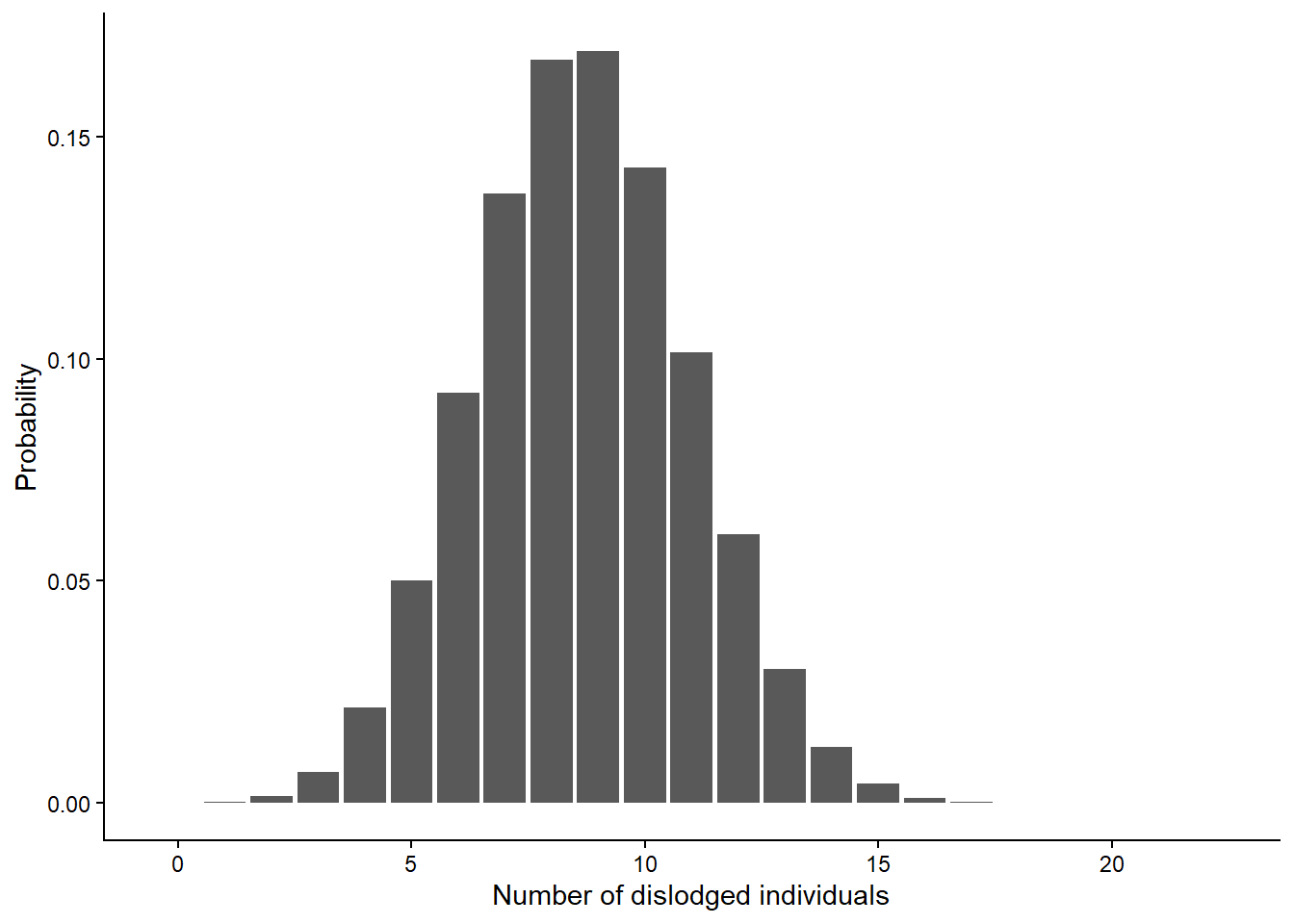

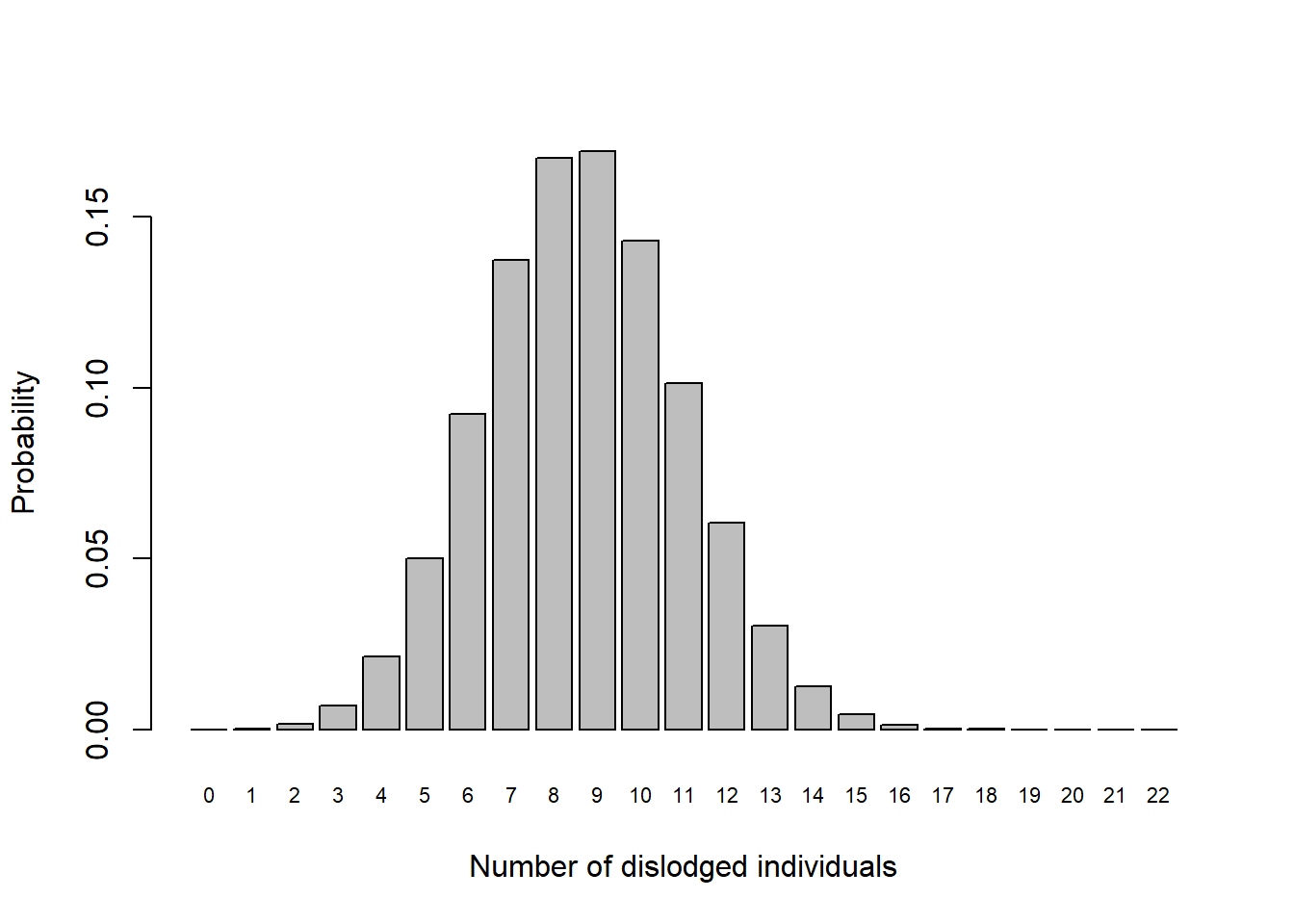
Bar plot (base R)

barplot(dbinom(0:k, k, p), 
        names.arg=0:k, 
        xlab="Number of dislodged individuals",
        ylab="Probability", 
        cex.names=0.7) # Changes the size of the 'names' (default = 1)

What is the probability that 9 individuals are dislodged?

P(y = 9 | p, k)

dbinom(9, k, p)

[1] 0.1691739

What is the probability that 5 or fewer dislodge (\(\le 5\))?

P(y <= 5 | p, k)

sum(dbinom(0:5, k, p)) # pbinom(5, k, p)

[1] 0.08032148

How many out of every 10 years would you expect more than half of this population to dislodge (i.e., \(> 11\)), assuming dislodgement occurs independently among years?

P(y > 11 | p, k) * 10 years

10 * sum(dbinom(12:k, k, p))  # 1 - pbinom(11, k, p)

[1] 1.0928

Poisson distribution

Scenario 1

The Dogwhelks sheet from H2SMS_practicalData.xlsx contains the number of dog whelks (Nucella lapillus) in 40 quadrats on a beach on Skye. Load the dataset and calculate the mean and variance of the number of dog whelks per quadrat.

Load and check data

dw_df <- read_xlsx("data/H2SMS_practicalData.xlsx", sheet="Dogwhelks")
str(dw_df)

tibble [40 × 2] (S3: tbl_df/tbl/data.frame)
 $ quadrat   : num [1:40] 1 2 3 4 5 6 7 8 9 10 ...
 $ num_whelks: num [1:40] 0 1 0 0 0 2 1 2 0 0 ...

Calculate mean and variance

mean(dw_df$num_whelks)
var(dw_df$num_whelks)

[1] 0.6
[1] 0.5025641

What is the proportion of quadrats with 0, 1, and 2 dogwhelks?

Proportions: Method 1

mean(dw_df$num_whelks == 0)
mean(dw_df$num_whelks == 1)
mean(dw_df$num_whelks == 2)

[1] 0.525
[1] 0.35
[1] 0.125

Proportions: Method 2

dw_df |>
  count(num_whelks) |> # count occurrences of each value, put in new column `n`
  mutate(proportion=n/sum(n))

# A tibble: 3 × 3
  num_whelks     n proportion
       <dbl> <int>      <dbl>
1          0    21      0.525
2          1    14      0.35 
3          2     5      0.125

Proportions: Method 3

table(dw_df$num_whelks)/nrow(dw_df) # table() counts occurrences of each value


    0     1     2 
0.525 0.350 0.125

Using the sample mean as \(\lambda\), what is the probability of observing more than 2 dogwhelks in the next quadrat?

P(y > 2 | lambda)

lambda <- mean(dw_df$num_whelks)
1 - ppois(2, lambda)

[1] 0.02311529

If you were to repeat the sampling (\(n=40\) quadrats), in how many would you expect 1 dogwhelk?

P(y = 1 | lambda) * 40 quadrats

dpois(1, lambda) * 40

[1] 13.17148

Scenario 2

In July from 2018-2022, there were an average of 14.2 days where an orca sighting was reported in Shetland (shetland.org).

For the following questions, use the Poisson distribution to approximate the distribution of the number of days with reported sightings. Assume that the days with reported sightings occur independently and that there is no change in methodology or ecology.

What is the probability that there are 7 or fewer days with reported sightings next July?

P(y <=7 | lambda)

lambda <- 14.2
ppois(7, lambda)

[1] 0.02831033

What is the probability of having 14 days with sightings?

P(y = 14 | lambda)

dpois(14, lambda)

[1] 0.1058393

What is the probability of having 14 or more days with sightings?

P(y >= 14 | lambda)

1 - ppois(13, lambda)

[1] 0.5565904

What is the maximum possible number of days with sightings?

Maximum possible

# 31 days

According to the Poisson distribution, what is more likely: a July with 0 days with reported sightings or a July with more than 31 days of reported sightings?

P(y = 0 | lambda)

dpois(0, lambda)

[1] 6.807981e-07

P(y > max | lambda)

1 - ppois(31, lambda)

[1] 3.341259e-05

Interpretation

# There is a 0.00007% chance of 0 days with sightings and a
# 0.003% chance of >31 days with sightings.

# Remember to always consider the limits of your model!